Functionality of the fitbitViz R package
Lampros Mouselimis
2026-04-27
Source:vignettes/fitbit_viz.Rmd
fitbit_viz.RmdThe purpose of this Vignette is to show the main functionality of the
fitbitViz R package. Starting with version
1.0.8 the package no longer connects to the Fitbit Web
API — all functions accept pre-downloaded data
directly. The examples below use the bundled .RDS fixture
files from inst/tests_vignette_rds/ which are loaded
automatically in the setup chunk above.
We can now define the remaining variables,
WEEK <- 11 # for this use case pick the 11th week of the year 2021

weeks_2021 <- fitbitViz:::split_year_in_weeks(year = 2021) # split a year in weeks

# Start the week at monday (see: https://github.com/tidyverse/lubridate/issues/509)
date_start <- lubridate::floor_date(lubridate::ymd(weeks_2021[WEEK]), unit = "weeks") + 1

# Add 6 days to the 'date_start' variable to come to a 7-days plot
date_end <- date_start + 6

sleep_time_begins <- "00H 40M 0S"
sleep_time_ends <- "08H 00M 0S"

VERBOSE <- FALSE # disable verbosity
The previous code snippet uses one week of my personal Fitbit data (the 11th week of 2021) to plot my
- heart rate time series
- heart rate heatmap
- heart rate variability during sleep time
- sleep time series
- GPS data of outdoor activities
- 3-dimensional map of activities
The data for all these functions are available to download using the csv buttons in this Rmarkdown file.
heart rate time series
The heart_rate_time_series() function accepts the heart_rate_intraday_list (a named list of intraday data.tables, one per date) and an optional heart_rate summary data.frame, along with the detail level (1 minute), and returns the heart rate time series. Each output plot (of the multiplot) includes in the x-axis the time and in the y-axis the heart rate value. The highest heart rate value (peak) of the day is highlighted using a vertical and horizontal blue line,
# .......................
# heart rate time series
# .......................

heart_dat <- fitbitViz::heart_rate_time_series(
  heart_rate_intraday_list = heart_dat$heart_rate_intraday,
  heart_rate = heart_dat$heart_rate,
  detail_level = "1min",
  ggplot_intraday = TRUE,
  ggplot_ncol = 2,
  ggplot_nrow = 4,
  verbose = VERBOSE
)
heart_dat$plt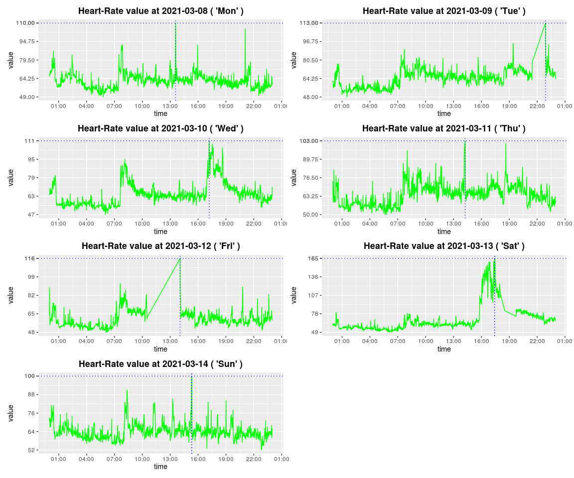
heart rate heatmap
The heart rate heatmap shows the min, median and max heart rate Levels in the y-axis for each day of the specified week (x-axis). As the legend shows, the displayed values range from 40 to 220 and higher values appear in purple or orange color,
# ............................
# heart rate intraday heatmap [ plot options: https://yihui.org/knitr/options/#plots ]
# ............................

heart_intra <- heart_dat$heart_rate_intraday

hrt_heat <- fitbitViz::heart_rate_heatmap(
  heart_rate_intraday_data = heart_intra,
  angle_x_axis = 0
)
hrt_heat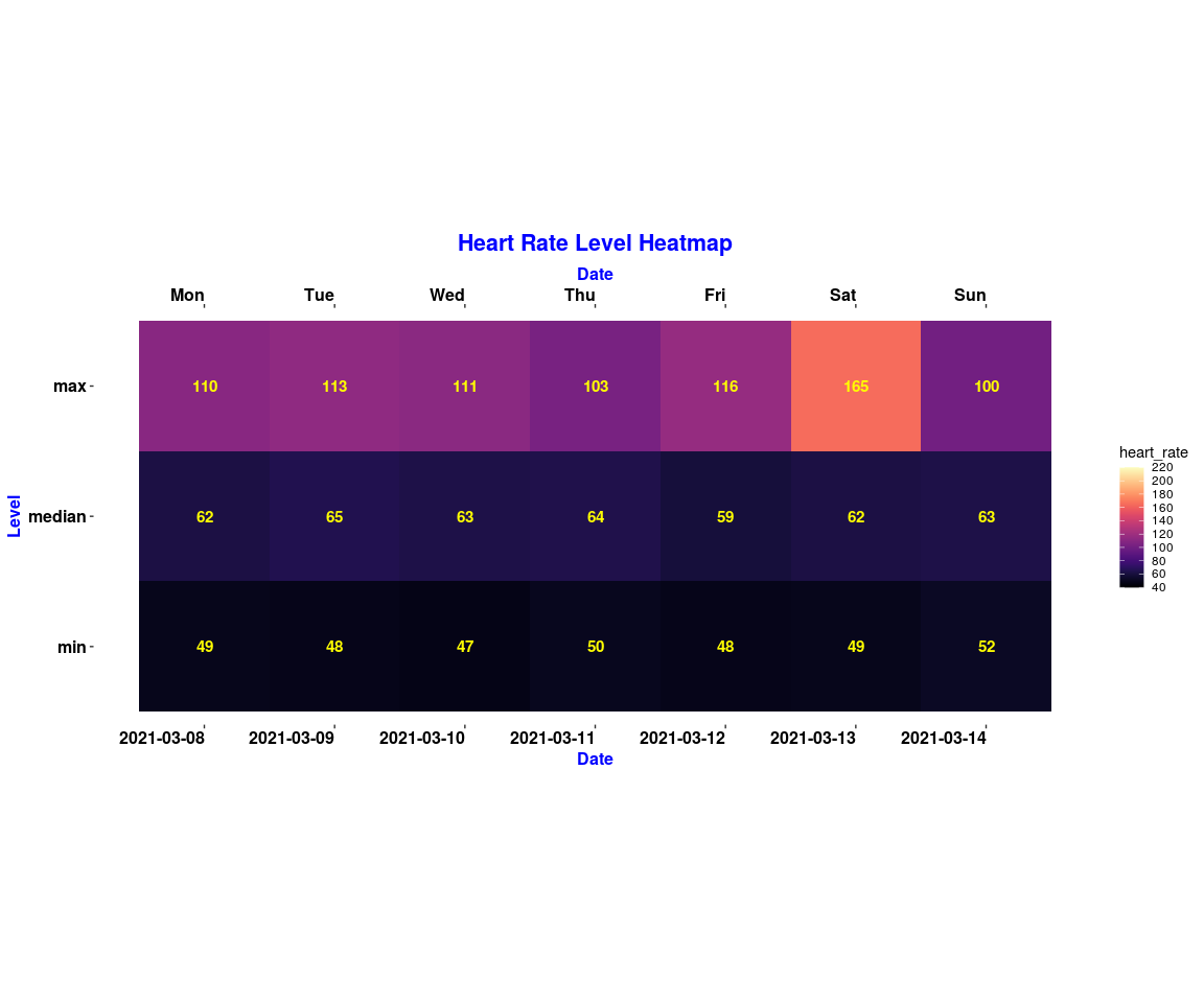
heart rate variability during sleep time
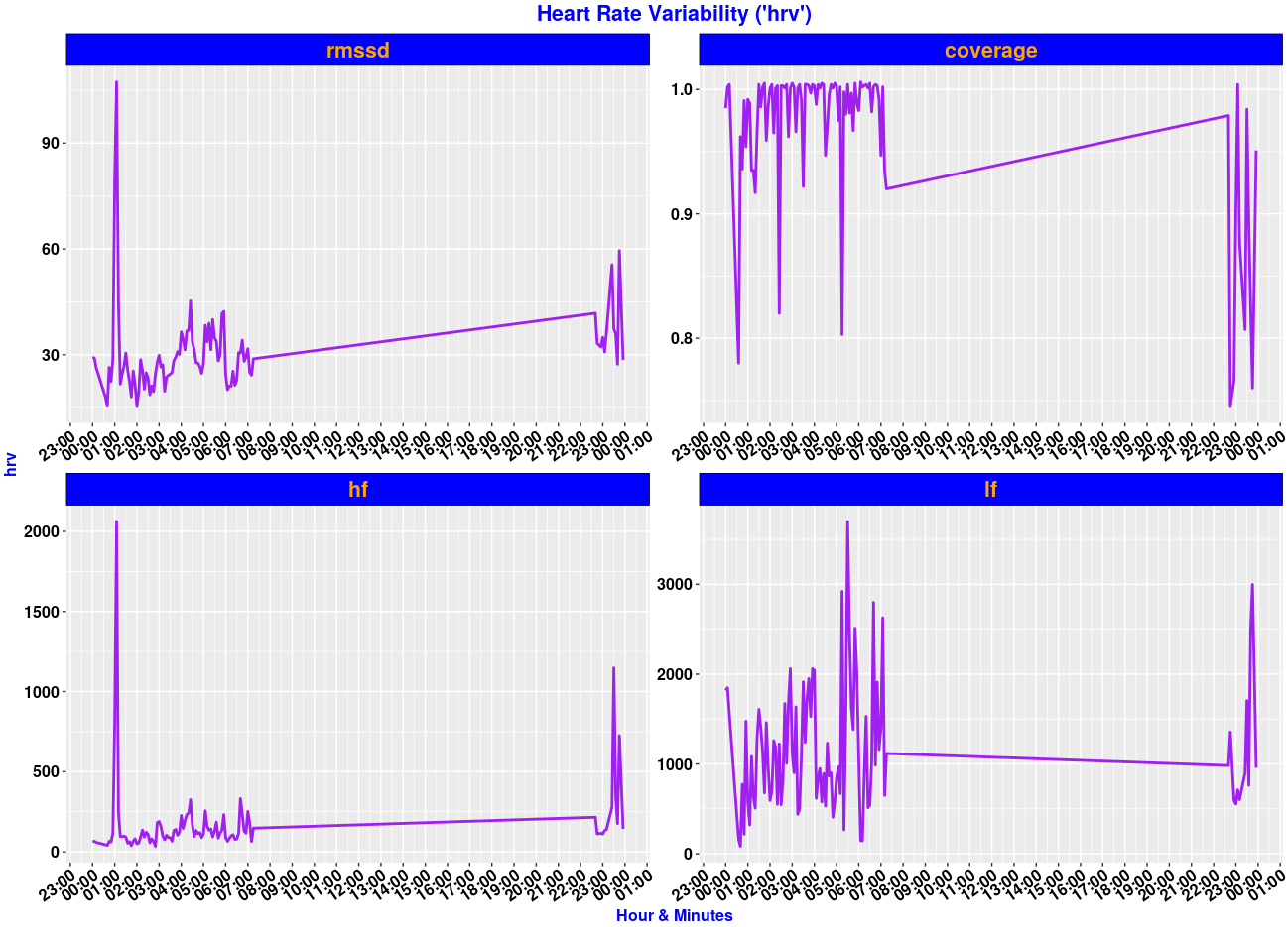
Heart Rate Variability (HRV) intraday data for a single date. HRV data applies specifically to a user’s “main sleep”, which is the longest single period of time asleep on a given date. It measures the HRV rate at various times and returns the Root Mean Square of Successive Differences (rmssd), Low Frequency (LF), High Frequency (HF), and Coverage data for a given measurement. Rmssd measures short-term variability in your heart rate while asleep. LF and HF capture the power in interbeat interval fluctuations within either high frequency or low frequency bands. Finally, coverage refers to data completeness in terms of the number of interbeat intervals. The fitbit_data_type_by_date() function allows the user to also compute the ‘spo2’ (Blood Oxygen Saturation), ‘br’ (Breathing Rate), ‘temp’ (Temperature) and ‘cardioscore’ (Cardio Fitness Score or VO2 Max) by adjusting the type parameter.
# .......................
# heart rate variability
# .......................

hrt_rt_var <- fitbitViz::fitbit_data_type_by_date(
  data = heart_dat,
  type = "hrv",
  plot = TRUE
)
sleep time series
The sleep time series visualization is similar to the Fitbit Mobile Visualization and in the x-axis shows the specified by the user sleep time interval whereas in the y-axis shows the sleep Levels (wake, rem, light, deep). Lower levels like deep sleep appear in dark blue whereas higher levels like wake appear in light blue,
# .......................
# sleep data time series
# .......................

sleep_ts <- fitbitViz::sleep_time_series(
  sleep_data_list = sleep_ts,
  ggplot_color_palette = "ggsci::blue_material",
  ggplot_ncol = 2,
  ggplot_nrow = 4,
  verbose = VERBOSE
)
sleep_ts$plt_lev_segments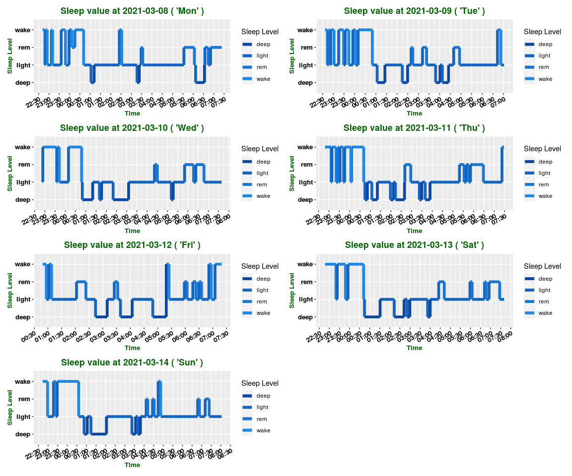
GPS data of outdoor activities
To make use of the GPS data from the Fitbit Application,
export the .tcx file for the desired activity from the
Fitbit website or app and pass its path to
GPS_TCX_data(),
# ....................................................
# return the gps-tcx data.table from an exported .tcx file
# ....................................................

res_tcx <- fitbitViz::GPS_TCX_data(
  tcx_file = "/path/to/activity.tcx",
  time_zone = "Europe/Athens",
  verbose = VERBOSE
)
# res_tcx
The following Leaflet Point Coordinates show my outdoor activity during the 11th week of 2021 (the legend shows the elevation of the route),
# ................................
# Create the Leaflet / LeafGL Map
# ................................

res_lft <- fitbitViz::leafGL_point_coords(
  dat_gps_tcx = res_tcx,
  color_points_column = "AltitudeMeters",
  provider = leaflet::providers$Esri.WorldImagery,
  option_viewer = rstudioapi::viewer,
  CRS = 4326
)
res_lft3-dimensional plots of activities
Another option of this package is to plot a route in 3-dimensional space. For this purpose we’ll use the rayshader package, which internally uses rgl (OpenGL). First, we have to extend the boundaries of our route for approximately 1.000 thousand meters (adjust this value depending on your area of interest),
# ...................................................
# compute the sf-object buffer and the raster-extend  (1000 meters buffer)
# ...................................................

sf_rst_ext <- fitbitViz::extend_AOI_buffer(
  dat_gps_tcx = res_tcx,
  buffer_in_meters = 1000,
  CRS = 4326,
  verbose = VERBOSE
)
# sf_rst_ext
Then for the extended area we will download Copernicus Digital Elevation Model (DEM) data. The Copernicus elevation data come either in 30 or in 90 meter resolution. We will pick the 30 meter resolution product for this route. The CopernicusDEM is an R package, make sure that you have installed and configured the awscli Operating System Requirement if you intend to download and reproduce the next 3-dimensional map using the elevation data,
# ..................................................................
# Download the Copernicus DEM 30m elevation data
# there is also the option to download the DEM 90m elevation data
# which is of lower resolution but the image size is smaller which
# means faster download
# ..................................................................

dem_dir <- tempdir()
# dem_dir

dem30 <- CopernicusDEM::aoi_geom_save_tif_matches(
  sf_or_file = sf_rst_ext$sfc_obj,
  dir_save_tifs = dem_dir,
  resolution = 30,
  crs_value = 4326,
  threads = parallel::detectCores(),
  verbose = VERBOSE
)

TIF <- list.files(dem_dir, pattern = ".tif", full.names = T)
# TIF

if (length(TIF) > 1) {
  # ....................................................
  # create a .VRT file if I have more than 1 .tif files
  # ....................................................

  file_out <- file.path(dem_dir, "VRT_mosaic_FILE.vrt")

  vrt_dem30 <- CopernicusDEM::create_VRT_from_dir(
    dir_tifs = dem_dir,
    output_path_VRT = file_out,
    verbose = VERBOSE
  )
}

if (length(TIF) == 1) {
  # ..................................................
  # if I have a single .tif file keep the first index
  # ..................................................

  file_out <- TIF[1]
}

# .......................................
# crop the elevation DEM based on the
# coordinates extent of the GPS-CTX data
# .......................................

raysh_rst <- fitbitViz::crop_DEM(
  tif_or_vrt_dem_file = file_out,
  sf_buffer_obj = sf_rst_ext$sfc_obj,
  verbose = VERBOSE
)
# terra::plot(raysh_rst)
The GPS route that I use is an ascending & descending route therefore we can convert the GPS (TCX) data to a spatial LINESTRING by using the maximum altitude as a split point of the route to visualize the ascending route in blue and the descending in red (there is also the alternative to specify the split point based on time using the time_split_asc_desc parameter),
linestring_dat <- fitbitViz::gps_lat_lon_to_LINESTRING(
  dat_gps_tcx = res_tcx,
  CRS = 4326,
  time_split_asc_desc = NULL,
  verbose = VERBOSE
)
then we create the ‘elevation_sample_points’ data.table parameter for the 3-dim plot based on the min., middle and max. altitude of the previously computed ‘res_tcx’ data,
idx_3m <- c(
  which.min(res_tcx$AltitudeMeters),
  as.integer(length(res_tcx$AltitudeMeters) / 2),
  which.max(res_tcx$AltitudeMeters)
)

cols_3m <- c("latitude", "longitude", "AltitudeMeters")
dat_3m <- res_tcx[idx_3m, ..cols_3m]
and finally we visualize the 3-dimensional Rayshader Map,
# .....................................................
# Conversion of the 'SpatRaster' to a raster object
# because the 'rayshader' package accepts only rasters
# .....................................................

rst_obj <- raster::raster(raysh_rst)
raster::projection(rst_obj) <- terra::crs(raysh_rst, proj = TRUE)


snapshot_rayshader_path <- file.path(tempdir(), "rayshader_img.png")

rgl::open3d(useNULL = TRUE) # this removes the second rgl-popup-window

fitbitViz::rayshader_3d_DEM(
  rst_buf = rst_obj,
  rst_ext = sf_rst_ext$raster_obj_extent,
  linestring_ASC_DESC = linestring_dat,
  elevation_sample_points = dat_3m,
  zoom = 0.3,
  windowsize = c(1000, 800),
  add_shadow_rescale_original = FALSE,
  verbose = TRUE
)

rgl::rgl.snapshot(snapshot_rayshader_path)
rgl::par3d(mouseMode = "trackball") # options: c("trackball", "polar", "zoom", "selecting")
rgl::rglwidget()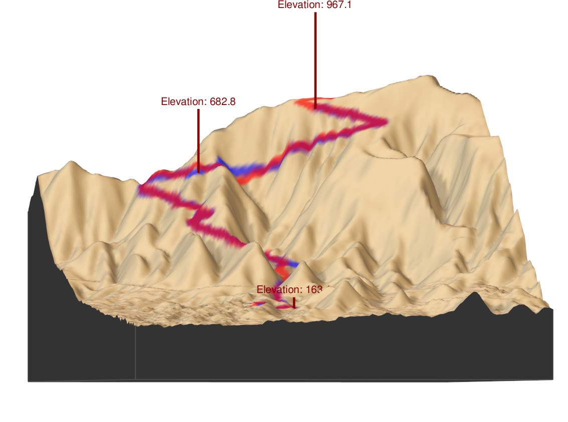
In the output map we observe
- the 3 specified elevation vertical lines (including their altitude values in meters)
- in blue color the ascending route
- in red color the descending route