ICESat-2 Virtual File System Orbits
Source:vignettes/IceSat-2_Virtual_File_System_Orbits_HTML.Rmd
IceSat-2_Virtual_File_System_Orbits_HTML.RmdIn this third vignette I’ll make use of the GDAL Virtual File Systems to download nominal and time specific orbit data (from the ICESat-2 Technical Specs website) for an Area of Interest (AOI). This will allow me to reduce the download and computation time once I make the requests to the OpenAltimetry API.
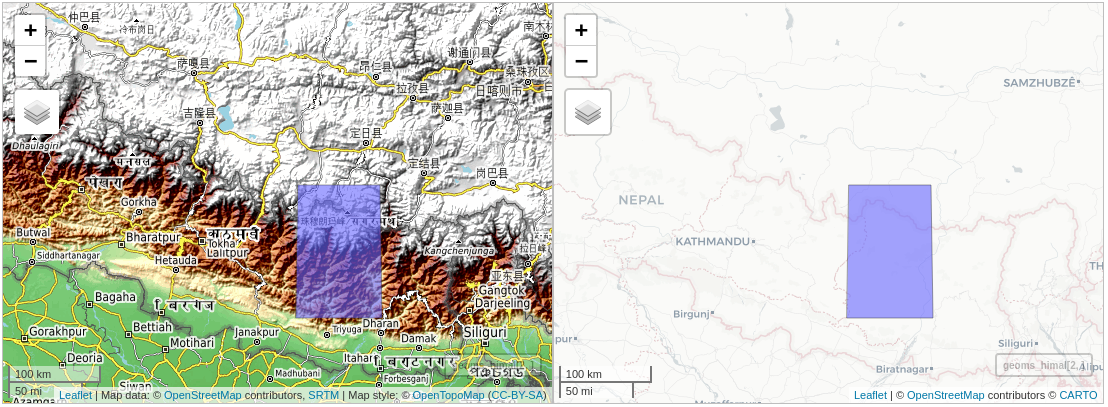
The area of interest is the Himalayas mountain range which has some of the highest peaks in the world, including mount Everest. The following map shows the bounding box area that I’ll use in this vignette,

Area of Interest
First, we load the data,
pkgs = c('IceSat2R', 'magrittr', 'sf', 'mapview', 'leaflet')
load_pkgs = lapply(pkgs, require, character.only = TRUE)  # load required R packages

geoms_himal_pth = system.file('data_files', 'vignette_data', 'himalayas.RDS', package = "IceSat2R")
geoms_himal = readRDS(geoms_himal_pth)
geoms_himal

# Simple feature collection with 2 features and 1 field
# Geometry type: POLYGON
# Dimension:     XY
# Bounding box:  xmin: 86.35254 ymin: 26.95635 xmax: 87.29736 ymax: 28.25842
# CRS:           EPSG:4326
#   area_size                       geometry
# 1     small POLYGON ((86.36902 27.66164...
# 2       big POLYGON ((86.35254 26.95635...
Since the Himalayas mountain range is located in the Eastern Hemisphere we’ll pick this as an area to use as input to the IceSat2R::vsi_nominal_orbits_wkt() function. Moreover, we’ll iterate over all 8 available repeats for the Eastern Hemisphere to retrieve the Reference Ground Tracks (RGTs) of the AOI based on the nominal orbits,
sf_wkt = sf::st_geometry(subset(geoms_himal, area_size == 'big'))

centr_wkt = sf::st_coordinates(sf::st_centroid(sf_wkt))
dat_wkt = sf::st_as_text(sf_wkt)

lst_out = list()

for (iter in 1:8) {         # iterate over all available repeats

  cat(paste0(iter, '.'))

  dat_iter = IceSat2R::vsi_nominal_orbits_wkt(orbit_area = 'eastern_hemisphere',
                                              track = 'GT7',
                                              rgt_repeat = iter,
                                              wkt_filter = dat_wkt,
                                              download_method = 'curl',
                                              download_zip = FALSE,
                                              verbose = TRUE)
  lst_out[[iter]] = dat_iter
}

# 1.The available Icesat-2 orbits will be red from 'https://icesat-2.gsfc.nasa.gov/ ...
# Access the data of the technical specs website ...
# Extract the .zip files and the corresponding titles ...
# Keep the relevant data from the url's and titles ...
# Process the nominal and time specific orbits separately ...
# Adjust the Dates of the time specific orbits ...
# Create the nominal orbits data.table ...
# Create the time specific orbits data.table ...
# Return a single data.table ...
# .............
# 8.The available Icesat-2 orbits will be red from 'https://icesat-2.gsfc.nasa.gov/ ...
# Access the data of the technical specs website ...
# .............
# Elapsed time: 0 hours and 0 minutes and 2 seconds.
# Data based on repeat and track will be kept ...
# Data based on repeat and track will be kept ...
# The file 'EasternHem_repeat8_GT7.kmz' will be processed ...
# Total Elapsed time: 0 hours and 0 minutes and 5 seconds.
lst_out = unlist(lst_out, recursive = F)
unq_rgts = as.vector(unique(unlist(lapply(lst_out, function(x) x$RGT))))
unq_rgts

 # [1] "96"   "157"  "363"  "538"  "599"  "805"  "866"  "1041" "1308" "1247"
For this specific use case we are interested in ICESat-2 data for a specific time period,
- from ‘2020-01-01’ to ‘2021-01-01’ (1-year’s data)
Therefore, we’ll make use of the IceSat2R::vsi_time_specific_orbits_wkt() function which queries all 15 ICESat-2 RGTs cycles (as of March 2022) to come to the RGTs intersection for the specified 1-year time interval,
date_start = '2020-01-01'
date_end = '2021-01-01'

orb_cyc_multi = IceSat2R::vsi_time_specific_orbits_wkt(date_from = date_start,
                                                       date_to = date_end,
                                                       RGTs = unq_rgts,
                                                       wkt_filter = dat_wkt,
                                                       verbose = TRUE)

# The available Icesat-2 orbits will be red from 'https://icesat-2.gsfc.nasa.gov/ ...
# Access the data of the technical specs website ...
# Extract the .zip files and the corresponding titles ...
# Keep the relevant data from the url's and titles ...
# Process the nominal and time specific orbits separately ...
# Adjust the Dates of the time specific orbits ...
# Create the nominal orbits data.table ...
# Create the time specific orbits data.table ...
# Return a single data.table ...
# Elapsed time: 0 hours and 0 minutes and 0 seconds.
# In total there are 5 intersected dates for which data will be processed!
# The RGT cycles from which data will be processed are:
#            RGT_cycle_6, RGT_cycle_7, RGT_cycle_8, RGT_cycle_9, RGT_cycle_10
# -------------------------------------------------
# RGTs of cycle 'RGT_cycle_6' will be processed ...
# -------------------------------------------------
# The 'sf' gdalinfo returned an empty character string! Attempt to read the url using
#      the OS configured 'gdalinfo' function ...
# The internal type of the .zip file is 'kml'
# The 'https://icesat-2.gsfc.nasa.gov/sites/default/files/page_files/IS2_RGTs_cycle6_...'
#      'zip'  file includes  1387  'kml' files.
# Elapsed time: 0 hours and 0 minutes and 8 seconds.
# 6 out of 10 sublists were empty and will be removed!
# -------------------------------------------------
# RGTs of cycle 'RGT_cycle_7' will be processed ...
# -------------------------------------------------
#
# .................
#
# -------------------------------------------------
# RGTs of cycle 'RGT_cycle_10' will be processed ...
# -------------------------------------------------
# The 'sf' gdalinfo returned an empty character string! Attempt to read the url using th ...
#       'gdalinfo' function ...
# The internal type of the .zip file is 'kml'
# The 'https://icesat-2.gsfc.nasa.gov/sites/default/files/page_files/IS2_RGTs_cycle10_date ...
#       'zip'  file includes  1387  'kml' files.
# Elapsed time: 0 hours and 0 minutes and 6 seconds.
# 6 out of 10 sublists were empty and will be removed!
# In total 5 RGT cycles will be included in the output 'sf' object (RGT_cycle_6, RGT_cycle_7,
#      RGT_cycle_8, RGT_cycle_9, RGT_cycle_10)!
# output of 'RGT_cycle_6' will be re-formatted ...
# The 'description' column of the output data will be processed ...
# output of 'RGT_cycle_7' will be re-formatted ...
# The 'description' column of the output data will be processed ...
# output of 'RGT_cycle_8' will be re-formatted ...
# The 'description' column of the output data will be processed ...
# output of 'RGT_cycle_9' will be re-formatted ...
# The 'description' column of the output data will be processed ...
# output of 'RGT_cycle_10' will be re-formatted ...
# The 'description' column of the output data will be processed ...
# Total Elapsed time: 0 hours and 2 minutes and 37 seconds.
The query returns 18 different Date-Time matches for our defined 1-year time period,
orb_cyc_multi

# Simple feature collection with 18 features and 14 fields
# Geometry type: POINT
# Dimension:     XY
# Bounding box:  xmin: 86.45225 ymin: 27.09347 xmax: 87.22874 ymax: 27.11331
# CRS:           EPSG:4326
# First 10 features:
#    .... drawOrder icon  RGT           Date_time day_of_year cycle                  geometry
# 1  ....        NA <NA>   96 2020-01-02 00:37:11           2     6 POINT (86.97015 27.10272)
# 2  ....        NA <NA>  538 2020-01-30 23:13:14          30     6 POINT (87.22874 27.09347)
# 3  ....        NA <NA>  599 2020-02-03 23:04:54          34     6 POINT (86.45225 27.11331)
# 4  ....        NA <NA> 1041 2020-03-03 21:40:57          63     6  POINT (86.71086 27.1045)
# 5  ....        NA <NA>   96 2020-04-01 20:17:02          92     7 POINT (87.09815 27.08729)
# 6  ....        NA <NA>  599 2020-05-04 18:44:45         125     7 POINT (86.58026 27.09789)
# 7  ....        NA <NA> 1041 2020-06-02 17:20:48         154     7 POINT (86.83886 27.08907)
# 8  ....        NA <NA>   96 2020-07-01 15:56:55         183     8 POINT (87.00215 27.09888)
# 9  ....        NA <NA>  538 2020-07-30 14:32:58         212     8 POINT (87.26075 27.08963)
# 10 ....        NA <NA>  599 2020-08-03 14:24:38         216     8 POINT (86.48426 27.10947)
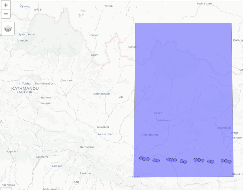
We’ll use the mapview R package to visualize our AOI bounding box with the intersected time-specific RGTs,
# make the sf-objects valid
orb_cyc_multi = sf::st_make_valid(orb_cyc_multi)
sf_wkt = sf::st_make_valid(sf_wkt)

# plot the sf-objects
orbit_cy = mapview::mapview(orb_cyc_multi, legend = F)
AOI_wkt = mapview::mapview(sf_wkt, legend = F)

lft = orbit_cy + AOI_wkt

lft = lft@map %>% leaflet::setView(lng = as.numeric(centr_wkt[, 'X']),
                                   lat = as.numeric(centr_wkt[, 'Y']),
                                   zoom = 7)
lft
Intersected RGTs
The output of ‘vsi_time_specific_orbits_wkt()’ can be verified with the OpenAltimetry’s ‘getTracks()’ function,
bbx_aoi = sf::st_bbox(obj = sf_wkt)

dtbl_rgts = verify_RGTs(nsidc_rgts = orb_cyc_multi,
                        bbx_aoi = bbx_aoi,
                        verbose = TRUE)
dtbl_rgts

#      Date_time RGT_OpenAlt RGT_NSIDC
#  1: 2020-01-02          96        96
#  2: 2020-01-30         538       538
#  3: 2020-02-03         599       599
#  4: 2020-03-03        1041      1041
#  5: 2020-04-01          96        96
#  6: 2020-05-04         599       599
#  7: 2020-06-02        1041      1041
#  8: 2020-07-01          96        96
#  9: 2020-07-30         538       538
# 10: 2020-08-03         599       599
# 11: 2020-09-01        1041      1041
# 12: 2020-09-30          96        96
# 13: 2020-11-02         599       599
# 14: 2020-12-01        1041      1041
# 15: 2020-12-30          96        96
# 16: 2021-01-28         538       538
# 17: 2021-02-01         599       599
# 18: 2021-03-02        1041      1041