
San Francisco Crime Classification competition
09 Jun 2016In this blog post, I’ll explain my approach for the San Francisco Crime Classification competition, in which I participated for the past two months. This competition was hosted by kaggle, a free online platform for predictive modelling and analytics. I ended up in the first 60 places out of 2335 participants and so far is my best personal result. This competition belongs to the knowledge competitions, meaning that the submissions of the participants are evaluated on the whole test data, so there wasn’t any danger of overfitting the leaderboard, as after every submission the true (end) leaderboard score was calculated (no secrets). Furthermore, there weren’t any ranking points, so no particular gain except for learning new methods on how to tackle machine learning problems.
the data set
The competition started one year ago, so there were some hints in the forum on how to exclude outliers or on how to approach this particular problem.
The dataset contained incidents derived from SFPD Crime Incident Reporting system and was collected from 1/1/2003 to 5/13/2015. The training set and test set rotated every week, meaning that week 1,3,5,7… belonged to test set whereas week 2,4,6,8 belonged to the training set. The following table shows the Category, which was the target of the competition,
train <- read.csv("train.csv", stringsAsFactors = F)

sort(table(train$Category), decreasing = T)


              LARCENY/THEFT              OTHER OFFENSES                NON-CRIMINAL                     ASSAULT
                     174900                      126182                       92304                       76876
              DRUG/NARCOTIC               VEHICLE THEFT                   VANDALISM                    WARRANTS
                      53971                       53781                       44725                       42214
                   BURGLARY              SUSPICIOUS OCC              MISSING PERSON                     ROBBERY
                      36755                       31414                       25989                       23000
                      FRAUD      FORGERY/COUNTERFEITING             SECONDARY CODES                 WEAPON LAWS
                      16679                       10609                        9985                        8555
               PROSTITUTION                    TRESPASS             STOLEN PROPERTY       SEX OFFENSES FORCIBLE
                       7484                        7326                        4540                        4388
         DISORDERLY CONDUCT                 DRUNKENNESS           RECOVERED VEHICLE                  KIDNAPPING
                       4320                        4280                        3138                        2341
DRIVING UNDER THE INFLUENCE                     RUNAWAY                 LIQUOR LAWS                       ARSON
                       2268                        1946                        1903                        1513
                  LOITERING                EMBEZZLEMENT                     SUICIDE             FAMILY OFFENSES
                       1225                        1166                         508                         491
                 BAD CHECKS                     BRIBERY                   EXTORTION   SEX OFFENSES NON FORCIBLE
                        406                         289                         256                         148
                   GAMBLING     PORNOGRAPHY/OBSCENE MAT                        TREA
                        146                          22                           6
The data can be downloaded directly from kaggle.
head(train)

               Dates       Category                       Descript DayOfWeek PdDistrict     Resolution
1 2015-05-13 23:53:00       WARRANTS                 WARRANT ARREST Wednesday   NORTHERN ARREST, BOOKED
2 2015-05-13 23:53:00 OTHER OFFENSES       TRAFFIC VIOLATION ARREST Wednesday   NORTHERN ARREST, BOOKED
3 2015-05-13 23:33:00 OTHER OFFENSES       TRAFFIC VIOLATION ARREST Wednesday   NORTHERN ARREST, BOOKED
4 2015-05-13 23:30:00  LARCENY/THEFT   GRAND THEFT FROM LOCKED AUTO Wednesday   NORTHERN           NONE
5 2015-05-13 23:30:00  LARCENY/THEFT   GRAND THEFT FROM LOCKED AUTO Wednesday       PARK           NONE
6 2015-05-13 23:30:00  LARCENY/THEFT GRAND THEFT FROM UNLOCKED AUTO Wednesday  INGLESIDE           NONE

                  Address         X        Y
        OAK ST / LAGUNA ST -122.4259 37.77460
        OAK ST / LAGUNA ST -122.4259 37.77460
 VANNESS AV / GREENWICH ST -122.4244 37.80041
  1500 Block of LOMBARD ST -122.4270 37.80087
 100 Block of BRODERICK ST -122.4387 37.77154
       0 Block of TEDDY AV -122.4033 37.71343


test <- read.csv("test.csv", stringsAsFactors = F)
head(test)

  Id               Dates DayOfWeek PdDistrict                  Address         X        Y
1  0 2015-05-10 23:59:00    Sunday    BAYVIEW  2000 Block of THOMAS AV -122.3996 37.73505
2  1 2015-05-10 23:51:00    Sunday    BAYVIEW       3RD ST / REVERE AV -122.3915 37.73243
3  2 2015-05-10 23:50:00    Sunday   NORTHERN   2000 Block of GOUGH ST -122.4260 37.79221
4  3 2015-05-10 23:45:00    Sunday  INGLESIDE 4700 Block of MISSION ST -122.4374 37.72141
5  4 2015-05-10 23:45:00    Sunday  INGLESIDE 4700 Block of MISSION ST -122.4374 37.72141
6  5 2015-05-10 23:40:00    Sunday    TARAVAL    BROAD ST / CAPITOL AV -122.4590 37.71317
I’ve red the data with stringsAsFactors = F, because I wanted the categorical columns to be in character and not in factor form, as I had to do some string preprocessing,
train = train[, -c(3,6)]
Furthermore, I removed the 3rd and 6th columns for two reasons: firstly they do appear only in the train data and secondly, I couldn’t find a way to take advantage of the Descript and Resolution.
train$Id = sort(seq(-nrow(train), -1, 1), decreasing = T)

test$Category = rep('none', nrow(test))

train = train[, c(8, 1:7)]

test = test[, c(1:2,8,3:7)]

train = rbind(train, test)
In order to horizontally join the train with the test data ( so that string preprocessing is feasible), I had to add an Id column to the train and a Category column to the test data. Then I shifted the order of columns so that the column names of the train data match the column names of the test data.
addr = train$Address

library(parallel)

rem_sl = unlist(mclapply(addr, function(x) stringr::str_replace(x, "/", ""), mc.cores = 4))

rem_sl1 = unlist(mclapply(rem_sl, function(x) stringr::str_replace_all(x, pattern=" ", repl=""), mc.cores = 4))

rem_sl2 = as.vector(sapply(rem_sl1, tolower))

train$Address = rem_sl2
To continue, I did some preprocessing of the Address column, as it appeared that some of these were in lower case, whereas others in upper case. First, I replaced c(‘/’, “ “) with an empty string “” and then I converted all addresses to lower case.
date = train$Dates


library(lubridate)

date1 = ymd_hms(date)

Year = year(date1)

Month = month(date1)

YDay = yday(date1)

WDay = wday(date1)

char_wdays = weekdays(date1)

Day = day(date1)

Hour = hour(date1)

Minute = minute(date1)
The Dates column was from a classification point of view important too, so I used the lubridate package to extract the year, month, yearsday, weekday (in numeric form), weekday (in character form),day, hour and minutes.
remov = data.frame(date_tmp = date1, order_dat = 1:length(date1))

remov1 = remov[order(remov$date_tmp, decreasing = F), ]

remov2 = cbind(remov1, order_out = 1:nrow(remov1))

remov3 = remov2[order(remov2$order_dat, decreasing = F), ]

ORD_rows = remov3$order_out
The training set and test set rotated every week, as I mentioned in the beginning, so I thought that a feature that tracks the order of the weeks could add some predictive power to the model,
library(zoo)

yq <- as.yearqtr(as.yearmon(as.Date(train$Dates), "%m/%d/%Y") + 1/12)

Season <- factor(format(yq, "%q"), levels = 1:4, labels = c("winter", "spring", "summer", "fall"))

Season = as.numeric(Season)

newy = which(Month == 1 & Day == 1)

newy1 = which(Month == 12 & Day == 31)

newal = rep(0, length(Month))

newal[newy] = 1

newal[newy1] = 1

train1 = data.frame(year = Year, month = Month, yday = YDay, weekday = WDay, day = Day, hour = Hour, minutes = Minute, season = Season, newy = newal, ORD_date = ORD_rows)

train1 = cbind(train, train1)
Furthermore, I utilized the zoo library to mark some periods of the year (seasons, new-year-event),
library(dplyr)

DISTRICTS = lapply(unique(train1$PdDistrict), function(x) filter(train1, PdDistrict == x))

median_outliers = function(sublist) {

  if (max(sublist$X) == -120.5 || max(sublist$Y) == 90.00) {

    sublist$X[which(sublist$X == -120.5)] = median(sublist$X)
    sublist$Y[which(sublist$Y == 90.00)] = median(sublist$Y)
  }

  sublist
}

distr = lapply(DISTRICTS, function(x) median_outliers(x))

distr1 = do.call(rbind, distr)
There were some potential outliers in the latitude and longitude data (X,Y columns), which should be replaced with the corresponding median of each district’s X and Y. Here, I used the filter function of the dplyr package as it was faster than the subset function of the base R.
address_frequency = function(sublist) {

  tmp_df = data.frame(table(sublist$Address))

  tmp_df = tmp_df[order(tmp_df$Freq, decreasing = T), ]

  tmp_df[1, ]$Var1
}


gcd.hf <- function(long1, lat1, long2, lat2) {                 # http://www.r-bloggers.com/great-circle-distance-calculations-in-r/

  R <- 6371                                               # Earth mean radius [km]

  delta.long <- (long2 - long1)

  delta.lat <- (lat2 - lat1)

  a <- sin(delta.lat/2) ^ 2 + cos(lat1) * cos(lat2) * sin(delta.long/2) ^ 2

  c <- 2 * asin(min(1,sqrt(a)))

  d = R * c

  return(d)                                                # Distance in km
}


get_reference_address = function(initial_data, split_column) {           # function to calculate km-distances

  s_col = lapply(unique(initial_data[, split_column]), function(x) initial_data[initial_data[, split_column] == x, ])

  reference_address = lapply(s_col, function(x) as.character(address_frequency(x)))

  reference_lon_lat = lapply(1:length(s_col), function(x) filter(s_col[[x]], Address == reference_address[[x]])[1, c('X','Y')])

  Distance = lapply(1:length(s_col), function(f) sapply(1:nrow(s_col[[f]]), function(x) gcd.hf(s_col[[f]][x, 7], s_col[[f]][x, 8],

                    reference_lon_lat[[f]]$X, reference_lon_lat[[f]]$Y)))

  tmp_id = do.call(rbind, s_col)$Id

  tmp_df = data.frame(id = tmp_id, unlist(Distance))

  colnames(tmp_df) = c('Id', paste('dist_', stringr::str_trim(split_column, side = 'both' )))

  return(tmp_df)
}


lst_out = list()

for (i in c('PdDistrict', 'weekday', 'day', 'hour', 'season')) {

  cat(i, '\n')

  lst_out[[i]] = get_reference_address(distr1, i)
}


merg = merge(lst_out[[1]], lst_out[[2]], by.x = 'Id', by.y = 'Id')

merg = merge(merg, lst_out[[3]], by.x = 'Id', by.y = 'Id')

merg = merge(merg, lst_out[[4]], by.x = 'Id', by.y = 'Id')

merg = merge(merg, lst_out[[5]], by.x = 'Id', by.y = 'Id')
The previous long code chunk takes advantage of the latitude and longitude data to calculate distance features. The idea behind the script was to spot, first, for each district (‘PdDistrict’) the locations with high crime frequency. Then, I extended the features by doing the same for ‘weekday’, ‘day’, ‘hour’ and ‘season’.
ndf = merge(distr1, merg, by.x = 'Id', by.y = 'Id')

ndf$`dist_ weekday` = log(ndf$`dist_ weekday` + 1)

ndf$`dist_ day` = sqrt(ndf$`dist_ day` + 1)

ndf$`dist_ hour` = 2 * sqrt(ndf$`dist_ hour` + 3/8)

ndf = ndf[, -c(2, 4)]
Then, I merged the distance-features (merg) with the initial data (distr1) and I took the log of the ‘dist_ weekday’, the sqrt of the ‘dist_ day’ and the Anscombe transform of the ‘dist_ hour’, as I observed some correlation of those transforms with the response variable. Additionally, I removed the 2nd (Dates) and 4th (DayOfWeek) columns, because Dates have been already preprocessed and the DayOfWeek appeared in numeric form already (weekday).
table(ndf$PdDistrict)

   BAYVIEW    CENTRAL  INGLESIDE    MISSION   NORTHERN       PARK   RICHMOND   SOUTHERN    TARAVAL TENDERLOIN
    179022     171590     158929     240357     212313      99512      90181     314638     132213     163556

pdD = as.factor(ndf$PdDistrict)

mdM = model.matrix(~.-1, data.frame(pdD))

ndf$PdDistrict = NULL

ndf = cbind(ndf, mdM)
I converted the PdDistrict predictor to dummy variables, as it didn’t have many Levels (like the Address column) and, in binarized form, it could add more predictive power to the model.
ndf$Address = as.numeric(as.factor(ndf$Address))

ntrain = filter(ndf, Id < 0)

ntrain$Id = NULL

response = ntrain$Category

y = c(0:38)[ match(response, sort(unique(response))) ]

ntrain$Category = NULL

ntest = filter(ndf, Id >= 0)

ID_TEST = as.integer(ntest$Id)

ntest$Id = NULL

ntest$Category = NULL
Finally, I split the end-data (ndf2) to train and test, I converted the response variable (y) to numeric (0:38) (so that it is compatible with the xgboost algorithm) and I removed redundant columns from both train (the Id) and test (the Category).
library(Matrix)

ntrain = Matrix(as.matrix(ntrain), sparse = T)

ntest = Matrix(as.matrix(ntest), sparse = T)
Some of the columns are highly sparse, thus converting the data to a sparse matrix could speed up the training. For this purpose, I used the Matrix library.
xgboost algorithm
The purpose of the competition was to decrease the Multi-class log loss thus, I used a corresponding function (MultiLogLoss) and additionally I built a validation function, which I used internally to evaluate the folds in xgboost (VALID_FUNC).
VALID_FUNC = function(EVAL_METRIC, arg_actual, arg_predicted, inverse_order = FALSE) {

  if (inverse_order == TRUE) {

    args_list = list(arg_predicted, arg_actual)
  }

  else {

    args_list = list(arg_actual, arg_predicted)
  }

  result = do.call(EVAL_METRIC, args_list)

  result
}


MultiLogLoss = function (y_true, y_pred) {

  if (is.factor(y_true)) {

    y_true_mat <- matrix(0, nrow = length(y_true), ncol = length(levels(y_true)))

    sample_levels <- as.integer(y_true)

    for (i in 1:length(y_true)) y_true_mat[i, sample_levels[i]] <- 1

    y_true <- y_true_mat
  }

  eps <- 1e-15

  N <- dim(y_pred)[1]

  y_pred <- pmax(pmin(y_pred, 1 - eps), eps)

  MultiLogLoss <- (-1/N) * sum(y_true * log(y_pred))

  return(MultiLogLoss)
}
I used the xgboost algorithm because it works pretty well with big data and gives good results as well. I performed a 4-fold cross-validation and at each fold, I also predicted the test data. The following function was used to evaluate each fold and to get the predictions from the unknown test data,
xgboost_cv = function(RESP, data, TEST, repeats, Folds, idx_train = NULL, param, num_rounds, print_every_n  = 10,

                      early_stop = 10, maximize = FALSE, verbose = 1, EVAL_METRIC, set_seed = 2) {

  start = Sys.time()

  library(caret)
  library(xgboost)
  library(Metrics)

  out_ALL = list()

  for (j in 1:repeats) {

    cat('REPEAT', j, '\n')

    TEST_lst = PARAMS = PREDS_tr = PREDS_te = list()

    if (is.numeric(Folds)) {

      if (is.null(set_seed)) {

        sample_seed = sample(seq(1, 1000000, 1), 1)}

      else {

        sample_seed = set_seed
      }

      set.seed(sample_seed)
      folds = createFolds(RESP, k = Folds, list = TRUE)}

    else {

      if (is.null(idx_train)) stop(simpleError('give index of train data in form of a vector'))

      out_idx = 1:dim(data)[1]
      folds = lapply(1:length(Folds), function(x) out_idx[which(idx_train %in% Folds[[x]])])
    }

    tr_er <- tes_er <- rep(NA, length(folds))

    for (i in 1:length(folds)) {

      cat('fold', i, '\n')

      dtrain <- xgb.DMatrix(data = data[unlist(folds[-i]), ], label = RESP[unlist(folds[-i])])

      dtest <- xgb.DMatrix(data = data[unlist(folds[i]), ], label = RESP[unlist(folds[i])])

      watchlist <- list(train = dtrain, test = dtest)

      fit = xgb.train(param, dtrain, nround = num_rounds, print.every.n  = print_every_n, watchlist = watchlist,

            early.stop.round = early_stop, maximize = maximize, verbose = verbose)

      PARAMS[[i]] = list(param = param, bst_round = fit$bestInd)

      pred_tr = predict(fit, data[unlist(folds[-i]), ], ntreelimit = fit$bestInd)
      pred_tr = matrix(pred_tr, nrow =  dim(data[unlist(folds[-i]), ])[1], ncol = length(unique(y)), byrow = TRUE)

      pred_te = predict(fit, data[unlist(folds[i]), ], ntreelimit = fit$bestInd)
      pred_te = matrix(pred_te, nrow =  dim(data[unlist(folds[i]), ])[1], ncol = length(unique(y)), byrow = TRUE)

      tr_er[i] = VALID_FUNC(EVAL_METRIC, as.factor(RESP[unlist(folds[-i])]), pred_tr)
      tes_er[i] = VALID_FUNC(EVAL_METRIC, as.factor(RESP[unlist(folds[i])]), pred_te)

      tmp_TEST = matrix(predict(fit, TEST, ntreelimit = fit$bestInd), nrow =  dim(TEST)[1], ncol = length(unique(y)), byrow = TRUE)

      TEST_lst[[paste0('preds_', i)]] = tmp_TEST

      cat('---------------------------------------------------------------------------', '\n')

      save(tmp_TEST, file = paste('sfcc_', paste(sample(1:1000000000, 1), '_REPEAT_save.RDATA', sep = ""), sep = ""))

      gc()
    }

    out_ALL[[j]] = list(TEST_lst = TEST_lst, PARAMS = PARAMS, sample_seed = sample_seed, tr_er = tr_er,PREDS_tr = PREDS_tr,

                        PREDS_te = PREDS_te, tes_er = tes_er)

    cat('================================================================================================================', '\n')

    gc()
  }

  end = Sys.time()

  return(list(res = out_ALL, time = end - start))
}
I experimented with different parameter settings, but the following one is a good trade-off between running time and performance, as it runs in 2.89 hours and gives a leaderboard score of 2.238 Multi-class log-loss. To improve the leaderboard score in this competition I averaged 6 models with different parameter settings. I observed that a learning rate (eta) of 0.145 and a number of rounds (num_rounds) 320 gave the best results,
params = list("objective" = "multi:softprob", "eval_metric" = "mlogloss", "num_class" = 39, "booster" = "gbtree", "bst:eta" = 0.245,

              "subsample" = 0.7, "max_depth" = 7, "colsample_bytree" = 0.7, "nthread" = 6, "scale_pos_weight" = 0.0,

              "min_child_weight" = 0.0, "max_delta_step" = 1.0)


fit = xgboost_cv(y, ntrain, ntest, repeats = 1, Folds = 4, idx_train = NULL, params, num_rounds = 145, print_every_n = 5,

                early_stop = 10, maximize = FALSE, verbose = 1, MultiLogLoss)
Before, submitting the csv-predictions, I had to calculate the train and test error for each fold, then to average the predictions of the unknown test data and to add the column names of the sample submission (the column names had to be in the correct form, otherwise the submission wasn’t accepted, thus check.names = F when reading the data was necessary),
tr_er = unlist(lapply(fit$res, function(x) x$tr_er))

tes_er = unlist(lapply(fit$res, function(x) x$tes_er))

cat('log loss of train is :', mean(tr_er), '\n')

# log loss of train is : 1.952143

cat('log loss of test is :',  mean(tes_er), '\n')

# log loss of test is : 2.232479

lap = unlist(lapply(fit$res, function(x) x$TEST_lst), recursive = FALSE)

avg_dfs = (lap[[1]] + lap[[2]] + lap[[3]] + lap[[4]])/4

subms = data.frame(ID_TEST, avg_dfs)

sampleSubmission <- read.csv("sampleSubmission.csv", check.names = F)

colnames(subms) = colnames(sampleSubmission)

subms = subms[order(subms$Id, decreasing = F), ]

write.csv(subms, "xgb_post_submission_train_error_1_95_test_error_2_2324.csv", row.names=FALSE, quote = FALSE)
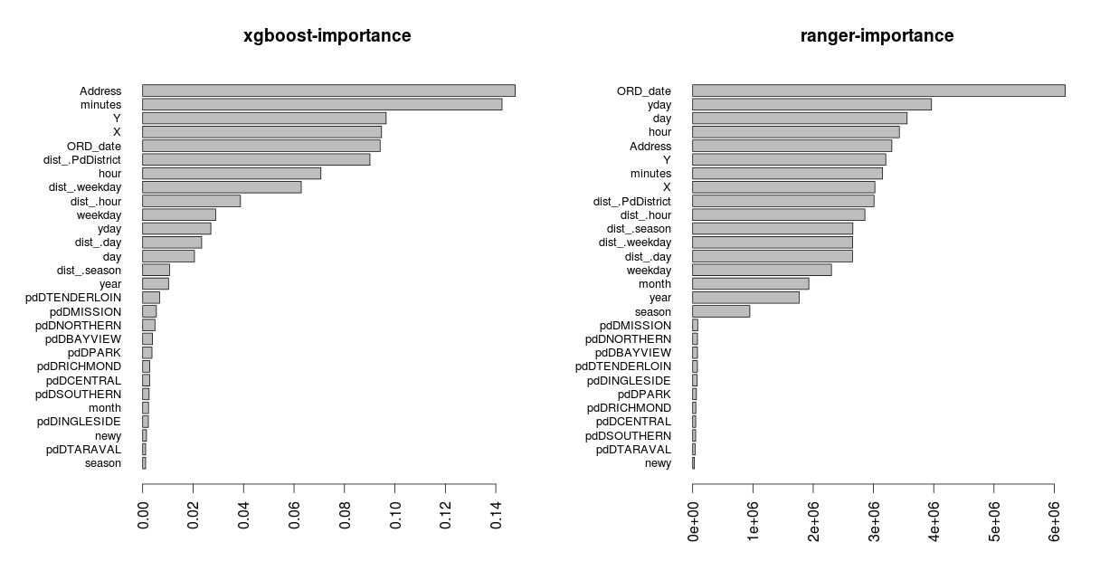
Finally, I’ll utilize the FeatureSelection package and especially xgboost and ranger to plot the important variables,
ntr = as.matrix(ntrain)

colnames(ntr) = make.names(colnames(ntr))


library(FeatureSelection)


params_xgboost = list(params = list("objective" = "multi:softprob", "eval_metric" = "mlogloss", "num_class" = 39, "booster" = "gbtree",

                                    "bst:eta" = 0.5, "subsample" = 0.65, "max_depth" = 5, "colsample_bytree" = 0.65, "nthread" = 6,

                                    "scale_pos_weight" = 0.0, "min_child_weight" = 0.0, "max_delta_step" = 1.0),

                      nrounds = 50, print.every.n = 5, verbose = 1, maximize = F)


params_ranger = list(write.forest = TRUE, probability = TRUE, num.threads = 6, num.trees = 50, verbose = FALSE, classification = TRUE,

                     mtry = 4, min.node.size = 5, importance = 'impurity')


params_features = list(keep_number_feat = NULL, union = F)


feat = wrapper_feat_select(ntr, y, params_glmnet = NULL, params_xgboost = params_xgboost, params_ranger = params_ranger, xgb_sort = NULL,

                           CV_folds = 4, stratified_regr = FALSE, cores_glmnet = 2, params_features = params_features)


params_barplot = list(keep_features = 28, horiz = TRUE, cex.names = 0.8)

barplot_feat_select(feat, params_barplot, xgb_sort = 'Cover')
The complete script of this blog post can be found as a single file in my Github account.