Feature Selection in R

This blog post is about feature selection in R, but first a few words about R. R is a free programming language with a wide variety of statistical and graphical techniques. It was created by Ross Ihaka and Robert Gentleman at the University of Auckland, New Zealand, and is currently developed by the R Development Core Team. R comes by installation with a core number of packages, which can be extended with more than 7,801 additional packages (as of January 2016). Packages can be downloaded from either the Comprehensive R Archive Network (CRAN) or from other sources like Github or the Bioconductor. Many of those statistical packages are written in R itself, however, a nice feature of R is that it can be linked to lower-level programming languages ( such as C or C++ ) for computationally intensive tasks. More information about R can be found here.

feature selection using lasso, boosting and random forest

There are many ways to do feature selection in R and one of them is to directly use an algorithm. This post is by no means a scientific approach to feature selection, but an experimental overview using a package as a wrapper for the different algorithmic implementations. I will make use of the glmnet, xgboost and ranger packages, because they work in high-dimensional data sets as well.

Glmnet is a package that fits a generalized linear model via penalized maximum likelihood. The regularization path is computed for the lasso or elasticnet penalty at a grid of values for the regularization parameter lambda. It fits linear, logistic, multinomial, poisson, and Cox regression models. The elastic-net penalty is controlled by α, and bridges the gap between lasso (α = 1, the default) and ridge (α = 0). The tuning parameter λ controls the overall strength of the penalty. It is known that the ridge penalty shrinks the coefficients of correlated predictors towards each other while the lasso tends to pick one of them and discard the others. The elastic-net penalty mixes these two. More info on the glmnet package can be found in the vignette.
In the FeatureSelection-wrapper package, it’s recommended that α is set to 1, because the main purpose is to keep the important predictors and remove all others. This is particularly useful in case of high-dimensional data or in data including many correlated predictors.

Xgboost stands for “Extreme Gradient Boosting” and is a fast implementation of the well known boosted trees. The tree ensemble model of xgboost is a set of classification and regression trees and the main purpose is to define an objective function and optimize it. Xgboost does an additive training and controls model complexity by regularization. More information on model and structure of xgboost can be found here. The xgboost algorithm orders the most important features by ‘Gain’, ‘Cover’ and ‘Frequency’. The gain gives an indication of the information of how a feature is important in making a branch of a decision tree more pure. Cover measures the relative quantity of observations concerned by a feature and Frequence counts the number of times a feature is used in all generated trees. In my wrapper package, the output is set by default to ‘Frequency’.

ranger is a fast implementation of random forest, particularly suited for high-dimensional data. Both random forest and boosted trees are tree ensembles, the only difference is that a random forest trains a number of trees and then these trees are averaged, whereas in boosting the learning of the next tree (N+1) depends on the previous tree (N). In the ranger package there are two different feature importance options, ‘impurity’ and ‘permutation’. Impurity is the improvement in the split-criterion at each split accumulated over all trees in the forest. The Permutation on the other hand is calculated after the tree is fitted by randomly shuffling each predictor’s data once at a time. The difference between the evaluation criterion before and after the shuffling gives the permutation importance. To expect is that important variables will be affected by this random sampling, whereas unimportant predictors will show minor differences.

Random forest feature selection has some drawbacks. For data including categorical variables with a different number of levels, random forests are biased in favor of those attributes with more levels, furthermore if the data contain groups of correlated features of similar relevance for the output, then smaller groups are favored over larger groups. Conditional inference trees, which use significance test procedures in order to select variables instead of selecting a variable that maximizes/minimizes an information measure, is a possible solution to the previous issues.

a wrapper package

To experiment with the previously mentioned algorithms, I have built a wrapper package called FeatureSelection, which can be installed from Github using install_github(‘mlampros/FeatureSelection’) of the devtools package. Furthermore, I will use the high-dimensional africa soil properties data from a past kaggle competition, which can be downloaded here. The purpose of the competition was to predict physical and chemical properties of soil using spectral measurements. The data came with a preprocessing script, which took the first derivatives to smooth out the measurement noise

trainingdata <- read.csv("~/training.csv")
MIR_measurements <- trainingdata[, 2:2655]
MIR_DER <- MIR_measurements- cbind(NA, MIR_measurements)[, -(dim(MIR_measurements)[2]+1)]
X_train <- cbind(trainingdata[, 3580:3595], MIR_DER[,-1])
MIR_measurements <- trainingdata[, 2671:3579]
MIR_DER <- MIR_measurements- cbind(NA, MIR_measurements)[, -(dim(MIR_measurements)[2]+1)]
X_train <- cbind(X_train, MIR_DER[, -1])
X_train$Depth = as.numeric(X_train$Depth)

Similarly, one could use the function gapDer of the prospectr package to calculate the Gap-Segment derivatives of the data, however I’ll continue with the former one. There were 5 target soil functional properties from diffuse reflectance infrared spectroscopy measurements to predict, but for the simplicity of the illustration I’ll proceed with a single one, i.e with the P target variable.

p = trainingdata[, 'P']

The FeatureSelection package comes with the following functions:

• primary
  • feature_selection (Feature selection for a single algorithm)
  • wrapper_feat_select (wrapper of all three methods)
• secondary
  • add_probs_dfs (addition of probability data frames)
  • barplot_feat_select (plots the important features)
  • class_folds (stratified folds (in classification))
  • func_shuffle (shuffle data)
  • normalized (normalize data)
  • regr_folds (create folds (in regression))
  • func_correlation
  • remove_duplic_func
  • second_func_cor
    

Once downloaded from Github one can view the details of each single function using ?, for instance ?feature_selection. To continue with the soil data set, I’ll use the wrapper_feat_select function in order to get the important features of all three algorithms,

library(FeatureSelection)

params_glmnet = list(alpha = 1, family = 'gaussian', nfolds = 5, parallel = TRUE)


params_xgboost = list( params = list("objective" = "reg:linear", "bst:eta" = 0.001, "subsample" = 0.75, "max_depth" = 5,
 
                                     "colsample_bytree" = 0.75, "nthread" = 6),
                      
                                      nrounds = 1000, print.every.n = 250, maximize = FALSE)
                       

params_ranger = list(dependent.variable.name = 'y', probability = FALSE, num.trees = 1000, verbose = TRUE, mtry = 5, 

                     min.node.size = 10, num.threads = 6, classification = FALSE, importance = 'permutation')


params_features = list(keep_number_feat = NULL, union = TRUE)


feat = wrapper_feat_select(X = X_train, y = p, params_glmnet = params_glmnet, params_xgboost = params_xgboost, 
 
                          params_ranger = params_ranger, xgb_sort = 'Gain', CV_folds = 5, stratified_regr = FALSE, 
                          
                          scale_coefs_glmnet = FALSE, cores_glmnet = 5, params_features = params_features, verbose = TRUE)

Each one of the params_glmnet, params_xgoobst and params_ranger takes arguments that are defined in the corresponding algorithm implementation. Recommended for glmnet is that alpha is always 1, so that feature selection is possible and in case of multiclass classification both thresh and maxit should be adjusted to reduce training time. For the ranger implementation it’s recommended in higher dimensions to use the dependent.variable.name and not the formula interface. The dependent.variable.name takes the response variable name as a string, however in order to make the FeatureSelection-wrapper work in all kind of data sets (high-dimensional as well), the dependent.variable.name will not equal the actual response variable name (here, ‘p’) but always the letter ‘y’. The additional params_features list takes two arguments, i.e. keep_number_feat if a certain number of the resulted important features should be kept and union, which ranks, normalizes, adds and then returns the importance of the features in decreasing order (experimental).

The resulted object of the wrapper_feat_select function can be a list of data frames if union is FALSE or a list of lists if union is TRUE, so in this case, it returns

str(feat)

List of 2
 $ all_feat  :List of 3
   $ glmnet-lasso:'data.frame':	102 obs. of  3 variables:
       $ Feature     : chr [1:102] "m1166.74" "m5939.75" "m2854.16" "m4431.67" ...
       $ coefficients: num [1:102] -30.8 -620.3 15.6 -175 -227 ...
       $ Frequency   : int [1:102] 5 5 4 4 4 4 4 3 3 3 ...
   $ xgboost     :'data.frame':	1245 obs. of  4 variables:
       $ Feature  : chr [1:1245] "m6975.34" "m1737.57" "BSAN" "m7492.18" ...
       $ Gain     : num [1:1245] 0.0793 0.0765 0.0407 0.0383 0.0376 ...
       $ Cover    : num [1:1245] 0.08372 0.03626 0.01889 0.00156 0.01793 ...
       $ Frequency: num [1:1245] 0.04739 0.02107 0.09184 0.01735 0.00939 ...
   $ ranger      :'data.frame':	3577 obs. of  2 variables:
       $ Feature    : Factor w/ 3577 levels "BSAN","BSAS",..: 174 311 1821 2176 1877 3113 327 1656 654 1498 ...
       $ permutation: num [1:3577] 0.00904 0.00826 0.00691 0.00658 0.00634 ...
 $ union_feat:'data.frame':	3577 obs. of  3 variables:
    $ feature   : Factor w/ 3577 levels "LSTN","m1159.02",..: 4 3 83 97 93 2 12 51 88 40 ...
    $ importance: num [1:3577] 1 0.961 0.813 0.787 0.787 ...
    $ Frequency : int [1:3577] 3 3 3 3 3 3 3 3 3 3 ...

The feature importance of the object feat can be plotted using the barplot_feat_select function, which takes as an additional argument the params_barplot,

params_barplot = list(keep_features = 30, horiz = TRUE, cex.names = 1.0)

barplot_feat_select(feat, params_barplot, xgb_sort = 'Cover')

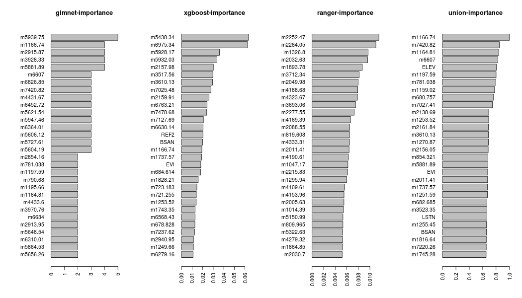
The keep_features, inside the params_barplot list, defines the number of features to be plotted and the horiz and cex.names are both arguments of the barplot function (details can be found in the graphics package).

correlation of variables

After the important features of each algorithm are returned, a next step could be to observe if the top features are correlated with the response and how each algorithm treated correlated predictors during feature selection.

The *func_correlation * function can be used here to return the predictors that are highly correlated with the response

dat = data.frame(p = p, X_train)

cor_feat = func_correlation(dat, target = 'p', correlation_thresh = 0.1, use_obs = 'complete.obs', correlation_method = 'pearson')

> head(cor_feat)
                 p
m781.038 0.1905918
m694.256 0.1830667
m696.184 0.1820458
m782.966 0.1801926
m802.251 0.1731508
m692.327 0.1719104

out_lst = lapply(feat$all_feat, function(x) which(rownames(cor_feat) %in% x[1:100, 1]))

> str(out_lst)
List of 3
 $ glmnet-lasso: int [1:9] 1 7 75 90 213 218 233 246 270
 $ xgboost     : int [1:22] 9 10 11 12 13 26 45 46 50 60 ...
 $ ranger      : int [1:29] 22 39 41 49 59 71 80 88 95 110 ...

It turns out that predictors highly correlated with the response appear in all methods as the out_lst object shows (taking into account the top 100 selected features). The same function func_correlation can be applied to reveal if multicollinearity is present in the top selected features of each method,

cor_lasso = func_correlation(X_train[, feat$all_feat$`glmnet-lasso`[, 1]], target = NULL, correlation_thresh = 0.9, 

                             use_obs = 'complete.obs', correlation_method = 'pearson')

> head(cor_lasso$out_df)
  predictor1 predictor2      prob
1   m1164.81   m1166.74 0.9782442
2   m1159.02   m1166.74 0.9010182
3   m2913.95   m2915.87 0.9275557
4    m4433.6   m4431.67 0.9812545
5   m4427.81   m4431.67 0.9762658
6   m1195.66   m1197.59 0.9850895

> dim(cor_lasso$out_df)[1]               # number of correlated pairs of predictors, lasso
[1] 10


cor_xgb = func_correlation(X_train[, feat$all_feat$xgboost[, 1][1:100]], target = NULL, correlation_thresh = 0.9, 

                           use_obs = 'complete.obs', correlation_method = 'pearson')

> head(cor_xgb$out_df)
  predictor1 predictor2      prob
1    m3608.2   m3610.13 0.9900190
2       BSAS       BSAN 0.9640673
3   m3523.35   m3517.56 0.9874395
4   m3525.28   m3517.56 0.9738908
5   m3434.64   m3517.56 0.9281257
6   m3432.71   m3517.56 0.9257304

> dim(cor_xgb$out_df)[1]               # number of correlated pairs of predictors, xgboost
[1] 82


cor_rf = func_correlation(X_train[, feat$all_feat$ranger[, 1][1:100]], target = NULL, correlation_thresh = 0.9,

                          use_obs = 'complete.obs', correlation_method = 'pearson')


> head(cor_rf$out_df)
  predictor1 predictor2      prob
1   m4796.15   m4828.94 0.9275590
2   m4836.65   m4828.94 0.9197116
3   m4350.67    m4352.6 0.9900792
4   m4344.89    m4352.6 0.9159542
5   m4354.53    m4352.6 0.9889634
6   m4358.38    m4352.6 0.9228754

> dim(cor_rf$out_df)[1]               # number of correlated pairs of predictors, ranger
[1] 32

The results show that all methods have correlated predictors in the top features (even the lasso, probably due to very high correlations among the predictors > 0.9), with xgboost having the most. In case of classification rather than calculating the correlation between features one can use the chisq.test in R to calculate the chi-squared statistic.

final word

This post was a small introduction to feature selection using three different algorithms. I used various functions from the wrapper-package FeatureSelection to show, how one can extract important features from data.