Comparison of Partition Around Medoid R programming Implementations
04 Dec 2022Back in September 2016 I implemented the ClusterR package. One of the algorithms included in ClusterR was the ‘Partition Around Medoids’ (Cluster_Medoids) algorithm which was based on the paper “Anja Struyf, Mia Hubert, Peter J. Rousseeuw, (Feb. 1997), Clustering in an Object-Oriented Environment, Journal of Statistical Software, Vol 1, Issue 4” (at that time I didn’t have access to the book of Kaufman and Rousseeuw, Finding Groups in Data (1990) where the exact algorithm was described), thus I implemented the code and compared my results with the output of the cluster::pam() function, which was available at that time. Thus, my method was not an exact but an approximate one. Recently, a user of the ClusterR package opened an issue mentioning that the results were not optimal compared to the cluster::pam() function and this allowed me to go through my code once again and also to compare my results to new R packages that were not existent at that time. Most of these R packages include a new version of the ‘Partition Around Medoids’ algorithm, “Erich Schubert, Peter J. Rousseeuw,”Faster k-Medoids Clustering: Improving the PAM, CLARA, and CLARANS Algorithms” 2019, <doi:10.1007/978-3-030-32047-8_16>”.
In this blog-post, I’ll use the following R packages,
to compare between the (as of December 2022) existing ‘Partition Around Medoids’ implementations in terms of output dissimilarity cost and elapsed time.
# required R packages

require(ClusterR)
## Loading required package: ClusterR

## Loading required package: gtools
require(cluster)
## Loading required package: cluster
require(kmed)
## Loading required package: kmed
require(fastkmedoids)
## Loading required package: fastkmedoids

##
## Attaching package: 'fastkmedoids'

## The following object is masked from 'package:cluster':
##
##     pam
require(sf)
## Loading required package: sf

## Linking to GEOS 3.7.1, GDAL 2.2.2, PROJ 4.9.2; sf_use_s2() is TRUE
require(data.table)
## Loading required package: data.table
require(geodist)
## Loading required package: geodist
require(glue)
## Loading required package: glue
require(magrittr)
## Loading required package: magrittr
require(ggplot2)
## Loading required package: ggplot2
require(mapview)
## Loading required package: mapview
require(knitr)
## Loading required package: knitr
Datasets
For comparison purposes, I’ll use the following datasets,
- a 2-column dataset using values of the Normal Distribution (standard deviation is equal to 0.25 and the mean parameter takes the value of 0 or 1)
- the ‘dietary_survey_IBS’ dataset which exists in the ClusterR package
- the ‘soybean’ dataset which exists in the ClusterR package
- the ‘agriculture’ dataset which exists in the cluster package
- a ‘geospatial’ dataset that shows how nicely the ‘Partition Around Medoids’ algorithm can cluster coordinate points based on a ‘geodesic’ distance matrix (assuming we can visually decide on the number of clusters)
The next function contains the previously mentioned datasets,
datasets_clust = function(data_name) {

  if (data_name == 'rnorm_data') {
    n = 100
    set.seed(1)
    x = rbind(matrix(rnorm(n, mean = 0, sd = 0.25), ncol = 2),
              matrix(rnorm(n, mean = 1, sd = 0.25), ncol = 2))
    lst_out = list(x = x, dataset = data_name)
  }
  else if (data_name == 'dietary_survey_IBS') {
    data(dietary_survey_IBS, package = 'ClusterR')
    x = dietary_survey_IBS[, -ncol(dietary_survey_IBS)]
    lst_out = list(x = x, dataset = data_name)
  }
  else if (data_name == 'soybean') {
    data(soybean, package = 'ClusterR')
    x = soybean[, -ncol(soybean)]
    lst_out = list(x = x, dataset = data_name)
  }
  else if (data_name == 'agriculture') {
    data(agriculture, package = 'cluster')
    x = agriculture
    lst_out = list(x = x, dataset = data_name)
  }
  else if (data_name == 'geospatial') {
    wkt_lst = list(black_sea = "POLYGON ((31.47957 43.64944, 31.47957 42.82356, 36.17885 42.82356, 36.17885 43.64944, 31.47957 43.64944))",
                   caspian_sea = "POLYGON ((49.23243 42.75324, 49.23243 41.99335, 51.54848 41.99335, 51.54848 42.75324, 49.23243 42.75324))",
                   mediterranean_sea = "POLYGON ((16.55062 35.08059, 16.55062 34.13804, 20.20771 34.13804, 20.20771 35.08059, 16.55062 35.08059))",
                   red_sea = "POLYGON ((36.61694 23.61829, 36.61694 22.60845, 38.18655 22.60845, 38.18655 23.61829, 36.61694 23.61829))")

    nam_wkts = names(wkt_lst)
    CRS_wkt = 4326
    sample_point_size = 250              # sample that many random points from each sea WKT polygon

    count = 1
    all_dfs = list()

    for (nam in nam_wkts) {
      WKT = wkt_lst[[nam]]
      read_wkt_inp = sf::st_as_sfc(WKT, crs = sf::st_crs(CRS_wkt))
      # to sample random points see:  https://stackoverflow.com/a/70073632/8302386
      random_lat_lons = sf::st_sample(x = read_wkt_inp, size = sample_point_size, type = "random", crs = sf::st_crs(CRS_wkt))
      random_df = sf::st_coordinates(random_lat_lons)
      random_df = data.table::as.data.table(random_df)
      colnames(random_df) = c('lon', 'lat')
      random_df$sea = rep(x = nam, times = nrow(random_df))
      random_df$code = rep(x = count, times = nrow(random_df))
      all_dfs[[count]] = random_df

      count = count + 1
    }

    dat = data.table::rbindlist(all_dfs)
    dat_sf = sf::st_as_sf(dat, coords = c('lon', 'lat'), crs = CRS_wkt)

    # add also an outlier which is between the 'mediterranean', 'black' and 'red' sea
    # and will be assigned to the one that is closest in terms of distance
    outlier_lon = 34.8988917972
    outlier_lat = 35.0385655983
    dat_sf_update = data.frame(lon = outlier_lon, lat = outlier_lat)

    x_mt_update = geodist::geodist(x = dat[, 1:2], y = dat_sf_update, measure = 'geodesic')
    x_mt_update = data.table::data.table(x_mt_update)
    x_mt_update$sea = dat$sea
    x_mt_update = x_mt_update[order(x_mt_update$V1, decreasing = F), ]

    dat_sf_update_obs = data.frame(lon = outlier_lon,
                                   lat = outlier_lat,
                                   sea = x_mt_update$sea[1],
                                   code = unique(subset(dat, sea == x_mt_update$sea[1])$code))   # it is assigned (based on distance) to the 'black sea' although it lies in the meditteranean
    dat_use = rbind(dat_sf_update_obs, dat)

    # leaflet map
    dat_sf_upd = sf::st_as_sf(dat_use, coords = c('lon', 'lat'), crs = CRS_wkt)
    mp = mapview::mapview(dat_sf_upd, zcol = 'sea', legend = TRUE)

    x = dat_use[, 1:2]
    lst_out = list(x = x,
                   dataset = data_name,
                   sea_names = dat_use$sea,
                   code = dat_use$code,
                   leaflet_map = mp)
  }
  else {
    stop(glue::glue("The dataset '{data_name}' does not exist!"), call. = FALSE)
  }

  return(lst_out)
}
‘Partion Around Medoids’ R package implementations
The next function includes the
- cluster::pam(do.swap = TRUE, variant = ‘original’)
- cluster::pam(do.swap = TRUE, variant = ‘faster’)
- kmed::skm()
- fastkmedoids::pam()
- fastkmedoids::fastpam(initializer = “LAB”)
- ClusterR::Cluster_Medoids(swap_phase = TRUE)
implementations and will allow comparing the dissimilarity cost and elapsed time for the mentioned datasets. In the ClusterR package, I included the ClusterR::cost_clusters_from_dissim_medoids() function that takes
- a dissimilarity matrix
- the output medoids of each implementation
and returns the total dissimilarity cost.
compare_medoid_implementations = function(x,
                                          y = NULL,
                                          max_k = 15,
                                          geodesic_dist = FALSE,
                                          round_digits = 5,
                                          compute_rand_index = FALSE) {
  if (!geodesic_dist) {
    x = ClusterR::center_scale(data = x, mean_center = TRUE, sd_scale = TRUE)
    x_mt = ClusterR::distance_matrix(x, method = "euclidean", upper = TRUE, diagonal = TRUE)
  }
  else {
    x_mt = geodist::geodist(x = x, measure = 'geodesic')
  }

  dv = as.vector(stats::dist(x))    # compute distance matrix for 'fastkmedoids' (lower triangular part)
  results = cluster_out = list()

  for (k in 2:max_k) {

    # cluster [ 'original' ]
    t_start = proc.time()
    set.seed(k)
    pm = cluster::pam(x = x_mt, k, metric = "euclidean", do.swap = TRUE, stand = FALSE, variant = 'original')
    pm_secs = as.numeric((proc.time() - t_start)["elapsed"])
    pm_cost = ClusterR::cost_clusters_from_dissim_medoids(data = x_mt, medoids = pm$id.med)$cost

    # cluster [ 'faster' ]
    t_start = proc.time()
    set.seed(k)
    pm_fast = cluster::pam(x = x_mt, k, metric = "euclidean", do.swap = TRUE, stand = FALSE, variant = 'faster')
    pm_fast_secs = as.numeric((proc.time() - t_start)["elapsed"])
    pm_fast_cost = ClusterR::cost_clusters_from_dissim_medoids(data = x_mt, medoids = pm_fast$id.med)$cost

    # kmed
    t_start = proc.time()
    km = kmed::skm(distdata = x_mt, ncluster = k, seeding = k, iterate = 10)
    km_secs = as.numeric((proc.time() - t_start)["elapsed"])
    km_cost = ClusterR::cost_clusters_from_dissim_medoids(data = x_mt, medoids = km$medoid)$cost

    # fastkmedoids  ('pam' function)
    t_start = proc.time()
    set.seed(k)
    fkm = fastkmedoids::pam(rdist = dv, n = nrow(x), k = k)
    fkm_secs = as.numeric((proc.time() - t_start)["elapsed"])
    fkm_cost = ClusterR::cost_clusters_from_dissim_medoids(data = x_mt, medoids = fkm@medoids + 1)$cost       # output indices correspond to Cpp indexing, thus add 1

    # fastkmedoids  ('fastpam' function with 'initializer' set to 'LAB')
    t_start = proc.time()
    fkm_lab = fastkmedoids::fastpam(rdist = dv, n = nrow(x), k = k, initializer = "LAB", seed = k)
    fkm_lab_secs = as.numeric((proc.time() - t_start)["elapsed"])
    fkm_lab_cost = ClusterR::cost_clusters_from_dissim_medoids(data = x_mt, medoids = fkm_lab@medoids + 1)$cost       # output indices correspond to Cpp indexing, thus add 1

    # ClusterR
    t_start = proc.time()
    clst = ClusterR::Cluster_Medoids(data = x_mt, clusters = k, verbose = FALSE, swap_phase = TRUE, seed = k)
    clst_secs = as.numeric((proc.time() - t_start)["elapsed"])
    clst_cost = ClusterR::cost_clusters_from_dissim_medoids(data = x_mt, medoids = clst$medoids)$cost

    clust_algos = c('cluster_pam',
                    'cluster_pam_fast',
                    'kmed_skm',
                    'fastkmedoids_pam',
                    'fastkmedoids_fastpam',
                    'ClusterR_Medoids')

    dissim_costs = c(round(pm_cost, digits = round_digits),
                     round(pm_fast_cost, digits = round_digits),
                     round(km_cost, digits = round_digits),
                     round(fkm_cost, digits = round_digits),
                     round(fkm_lab_cost, digits = round_digits),
                     round(clst_cost, digits = round_digits))

    time_bench = c(round(pm_secs, digits = round_digits),
                   round(pm_fast_secs, digits = round_digits),
                   round(km_secs, digits = round_digits),
                   round(fkm_secs, digits = round_digits),
                   round(fkm_lab_secs, digits = round_digits),
                   round(clst_secs, digits = round_digits))

    dtbl = list(pam_R_function = clust_algos,
                dissim_cost = dissim_costs,
                timing = time_bench,
                k = rep(k, length(clust_algos)))

    if (compute_rand_index) {
      # rand-index (or accuracy)
      clust_acc = list(k = k,
                       cluster_pam = ClusterR::external_validation(true_labels = y, clusters = pm$clustering, method = 'rand_index'),
                       cluster_pam_fast = ClusterR::external_validation(true_labels = y, clusters = pm_fast$clustering, method = 'rand_index'),
                       kmed_skm = ClusterR::external_validation(true_labels = y, clusters = km$cluster, method = 'rand_index'),
                       fastkmedoids_pam = ClusterR::external_validation(true_labels = y, clusters = fkm@assignment, method = 'rand_index'),
                       fastkmedoids_fastpam = ClusterR::external_validation(true_labels = y, clusters = fkm_lab@assignment, method = 'rand_index'),
                       ClusterR_Medoids = ClusterR::external_validation(true_labels = y, clusters = clst$clusters, method = 'rand_index'))

      data.table::setDT(clust_acc)
      cluster_out[[k]] = clust_acc
    }

    data.table::setDT(dtbl)
    results[[k]] = dtbl
  }

  results = data.table::rbindlist(results)

  if (compute_rand_index) {
    return(list(results = results, cluster_out = cluster_out))
  }
  else {
   return(results)
  }
}
In a for-loop, we’ll iterate over the datasets and the ‘partition around medoids’ implementations and we’ll save the output results to a list object,
dataset_names = c('rnorm_data', 'dietary_survey_IBS', 'soybean', 'agriculture', 'geospatial')
lst_all = list()
geo_flag = FALSE
y = NULL

for (dat_name in dataset_names) {

  iter_dat = datasets_clust(data_name = dat_name)
  cat(glue::glue("Dataset: '{dat_name}'  Number of rows: {nrow(iter_dat$x)}"), '\n')

  if (dat_name == 'geospatial') {
    mp_view = iter_dat$leaflet_map
    y = iter_dat$code
    geo_flag = TRUE
  }
  else {
    geo_flag = FALSE
  }

  iter_out = suppressWarnings(compare_medoid_implementations(x = iter_dat$x,
                                                             y = y,
                                                             max_k = 10,
                                                             geodesic_dist = geo_flag,
                                                             round_digits = 5,
                                                             compute_rand_index = geo_flag))
  lst_all[[dat_name]] = iter_out
}
## Dataset: 'rnorm_data'  Number of rows: 100
## Dataset: 'dietary_survey_IBS'  Number of rows: 400
## Dataset: 'soybean'  Number of rows: 307
## Dataset: 'agriculture'  Number of rows: 12
## Dataset: 'geospatial'  Number of rows: 1001
then we’ll use a ggplot2 visualization function to visualize the dissimilarity cost and elapsed time for each k from 2 to 10
multi_plot_data = function(data_index, y_column, digits = 2, size_geom_bar_text = 7) {

  data_index$k = factor(data_index$k)               # convert the 'k' column to factor
  levels(data_index$k) = as.factor(glue::glue("k = {levels(data_index$k)}"))
  data_index[[y_column]] = round(data_index[[y_column]], digits = digits)

  plt = ggplot2::ggplot(data_index, ggplot2::aes(x = factor(pam_R_function), y = .data[[y_column]], fill = factor(pam_R_function))) +
    ggplot2::geom_bar(stat = "identity") +
    ggplot2::facet_wrap(~k, scales = "free_y") +
    ggplot2::geom_text(ggplot2::aes(label = .data[[y_column]]), position = ggplot2::position_dodge(width = 0.9), col = 'black', fontface = 'bold', size = size_geom_bar_text) +
    ggplot2::theme(panel.background = ggplot2::element_rect(fill = "white", colour = "#6D9EC1", size = 3, linetype = "solid"),
          strip.text.x = ggplot2::element_text(size = 20, colour = 'black', face = 'bold'),
          strip.background = element_rect(fill = 'orange', colour = 'black'),
          plot.title = ggplot2::element_text(size = 19, hjust = 0.5),
          axis.text = ggplot2::element_text(size = 19, face = 'bold'),
          axis.text.x = ggplot2::element_text(size = 25, face = 'bold', angle = 35, hjust = 1),
          axis.title = ggplot2::element_text(size = 19, face = 'bold'),
          axis.title.x = ggplot2::element_blank(),
          panel.grid = ggplot2::element_blank(),
          legend.position = "none")

  return(plt)
}
Visualization of the dissimilarity cost for each one of the datasets
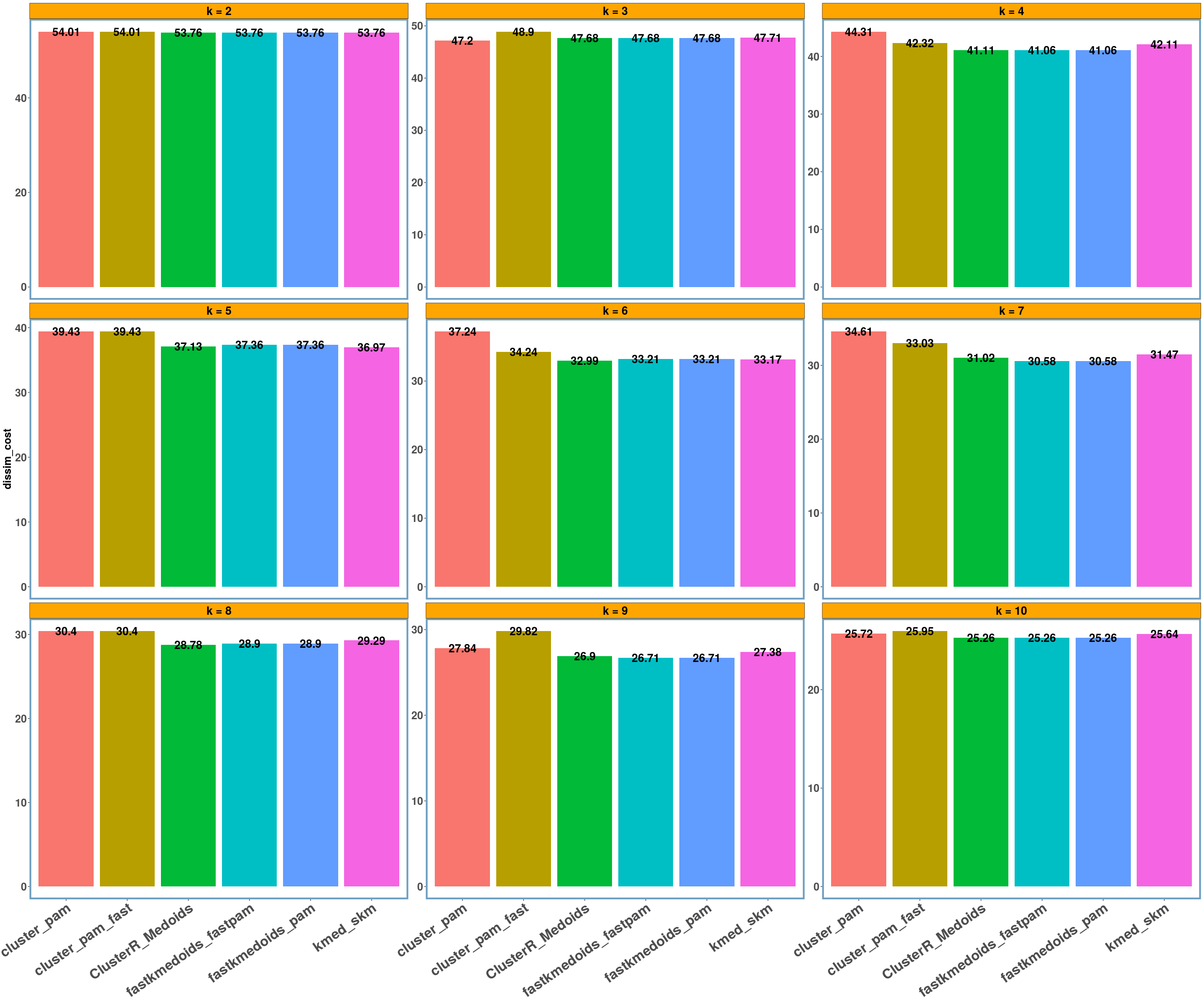
rnorm_data dataset
y_axis = 'dissim_cost'

data_name = 'rnorm_data'
multi_plot_data(data_index = lst_all[[data_name]], y_column = y_axis)
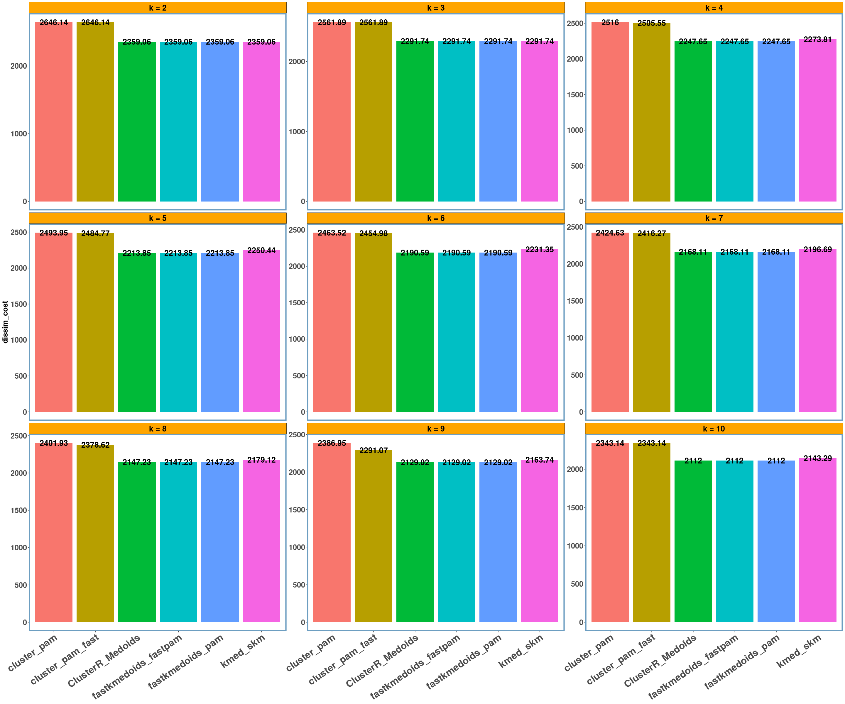
dietary_survey_IBS dataset
data_name = 'dietary_survey_IBS'
multi_plot_data(data_index = lst_all[[data_name]], y_column = y_axis)
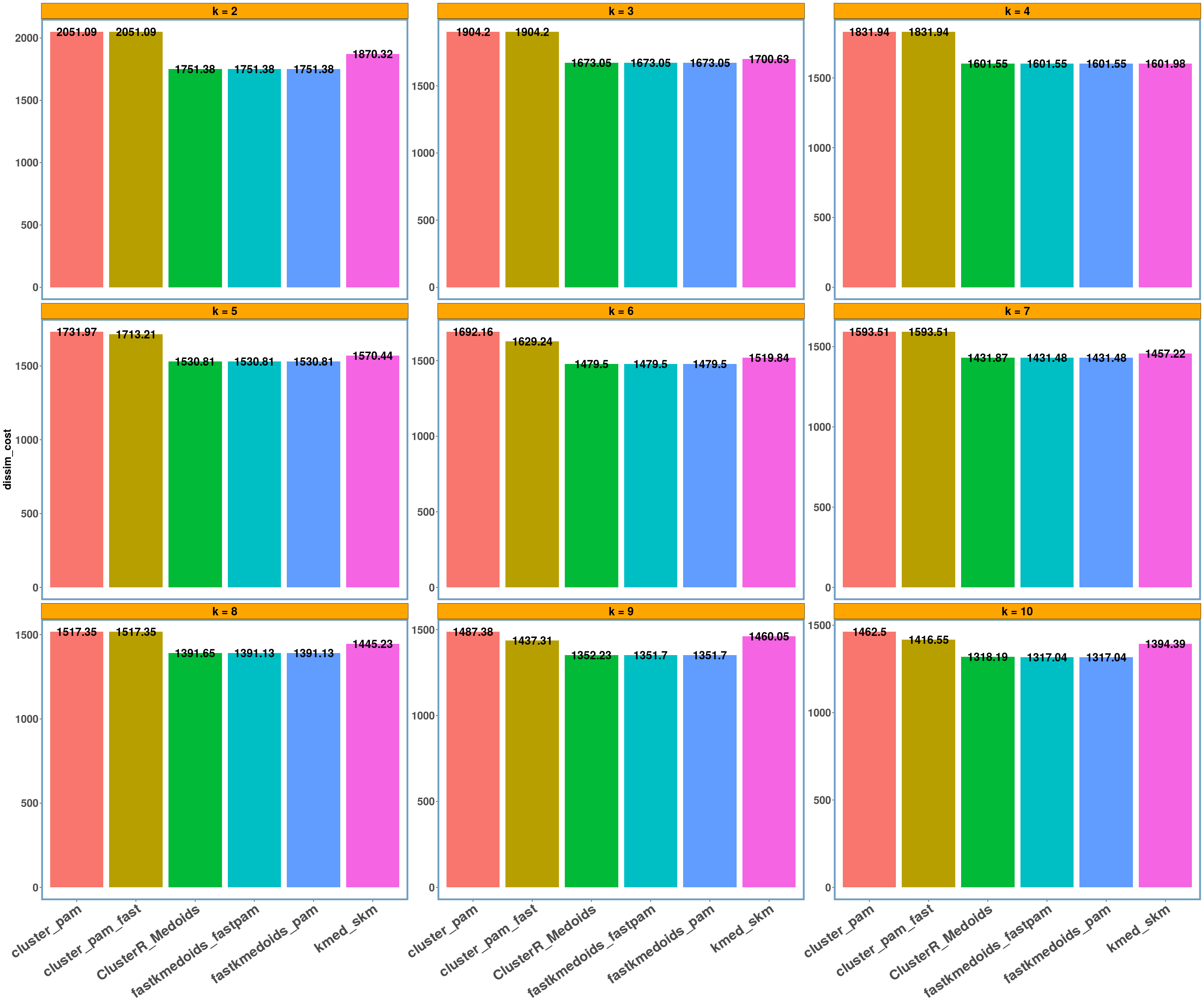
soybean dataset
data_name = 'soybean'
multi_plot_data(data_index = lst_all[[data_name]], y_column = y_axis)
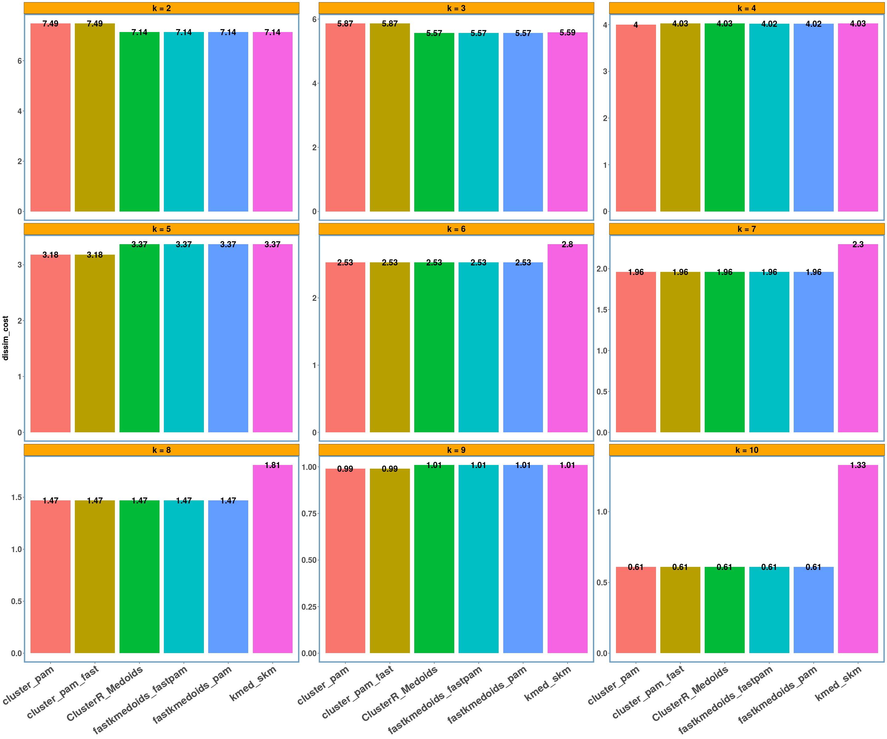
agriculture dataset
data_name = 'agriculture'
multi_plot_data(data_index = lst_all[[data_name]], y_column = y_axis)
geospatial dataset
data_name = 'geospatial'
multi_plot_data(data_index = lst_all[[data_name]]$results, y_column = y_axis, size_geom_bar_text = 5)
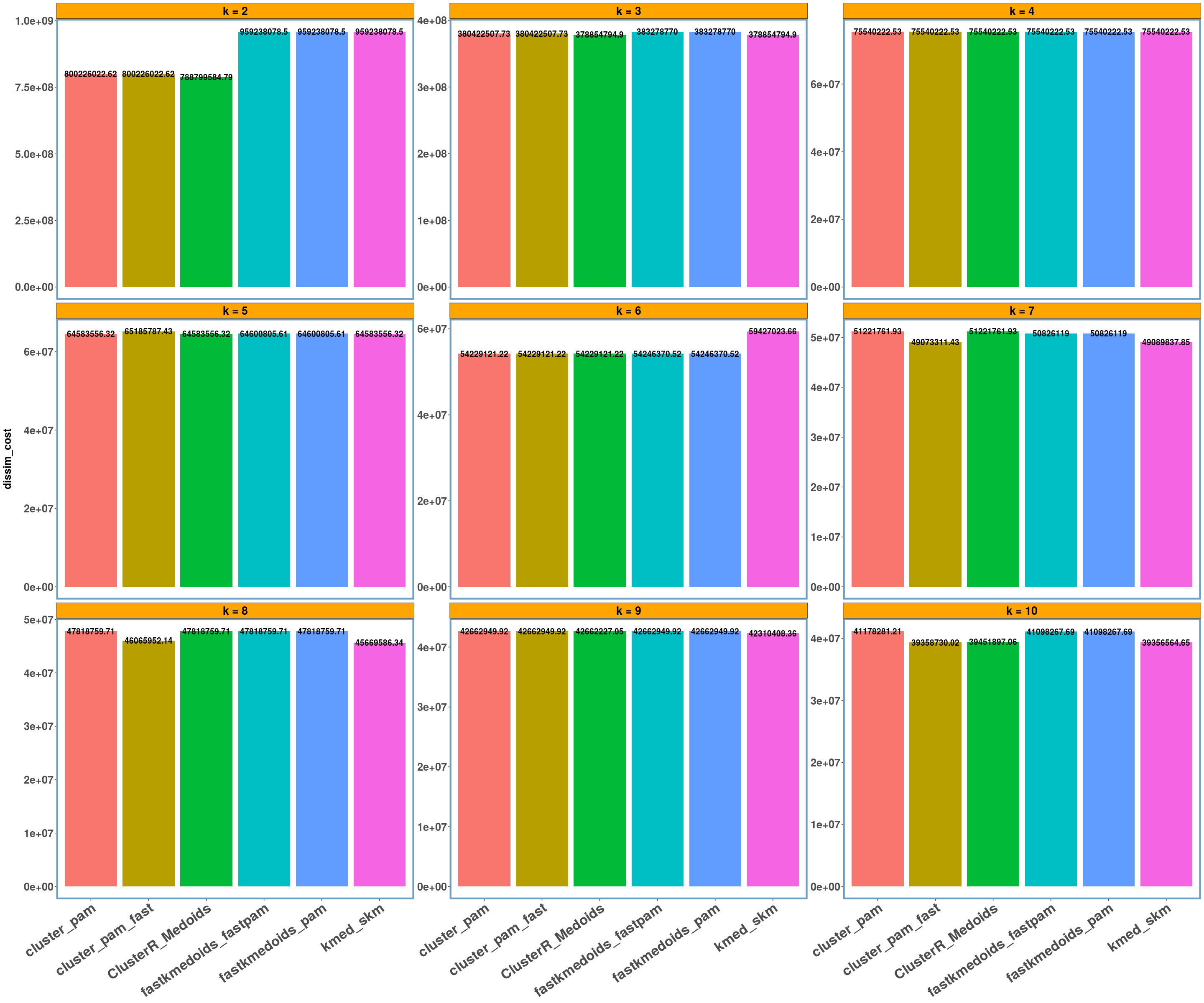
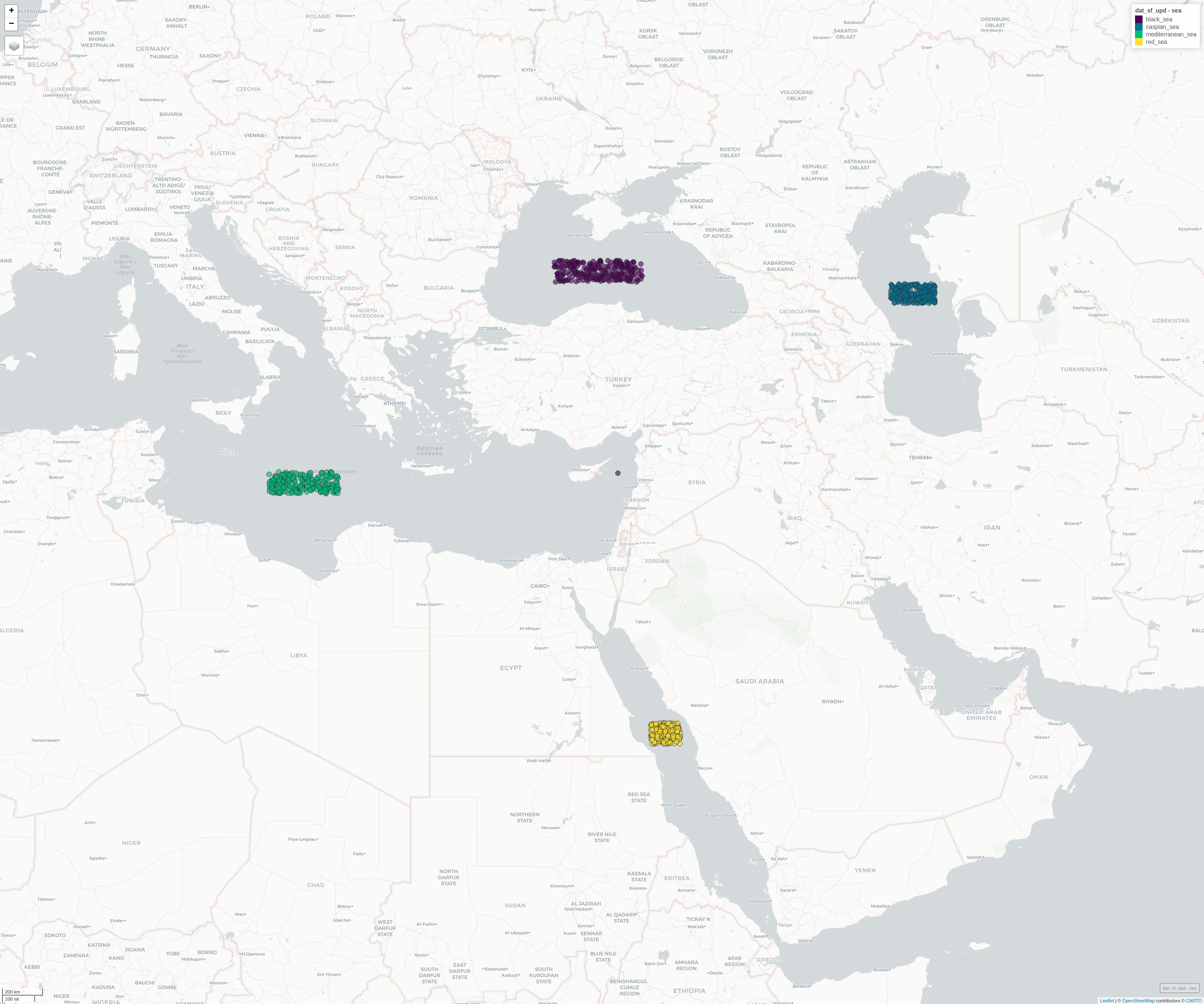
For the ‘geospatial’ data I also computed the Rand Index (or accuracy) and for k = 4 (which is the actual number of clusters as the following leaflet map shows) we have a perfect clustering (or a rand-index of 1.0). I also included a single outlier (a pair of coordinates) between the ‘mediterranean’, ‘black’ and ‘red’ sea, which shall be assigned to the ‘black’ sea based on the distance (which happens in all implementations),
dtbl_rand_index = data.table::rbindlist(lst_all[[data_name]]$cluster_out)
knitr::kable(round(dtbl_rand_index, digits = 3))
| k | cluster_pam | cluster_pam_fast | kmed_skm | fastkmedoids_pam | fastkmedoids_fastpam | ClusterR_Medoids |
|---|---|---|---|---|---|---|
| 2 | 0.624 | 0.624 | 0.624 | 0.624 | 0.624 | 0.624 |
| 3 | 0.874 | 0.874 | 0.875 | 0.846 | 0.846 | 0.875 |
| 4 | 1.000 | 1.000 | 1.000 | 1.000 | 1.000 | 1.000 |
| 5 | 0.969 | 0.969 | 0.969 | 0.969 | 0.969 | 0.969 |
| 6 | 0.938 | 0.938 | 0.937 | 0.938 | 0.938 | 0.938 |
| 7 | 0.927 | 0.906 | 0.907 | 0.927 | 0.927 | 0.927 |
| 8 | 0.917 | 0.896 | 0.896 | 0.917 | 0.917 | 0.917 |
| 9 | 0.886 | 0.886 | 0.865 | 0.885 | 0.885 | 0.885 |
| 10 | 0.875 | 0.854 | 0.855 | 0.875 | 0.875 | 0.855 |
The Leaflet map shows the 4 clusters of the geospatial dataset
which gives a rand-index of 1.0,
mp_view
Visualization of the elapsed time for each one of the datasets
rnorm_data dataset
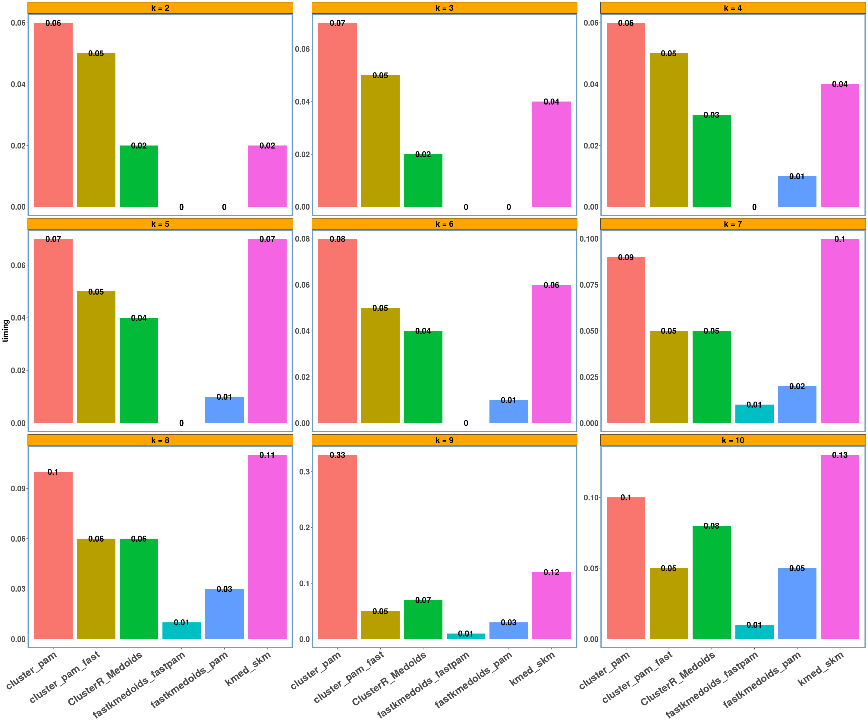
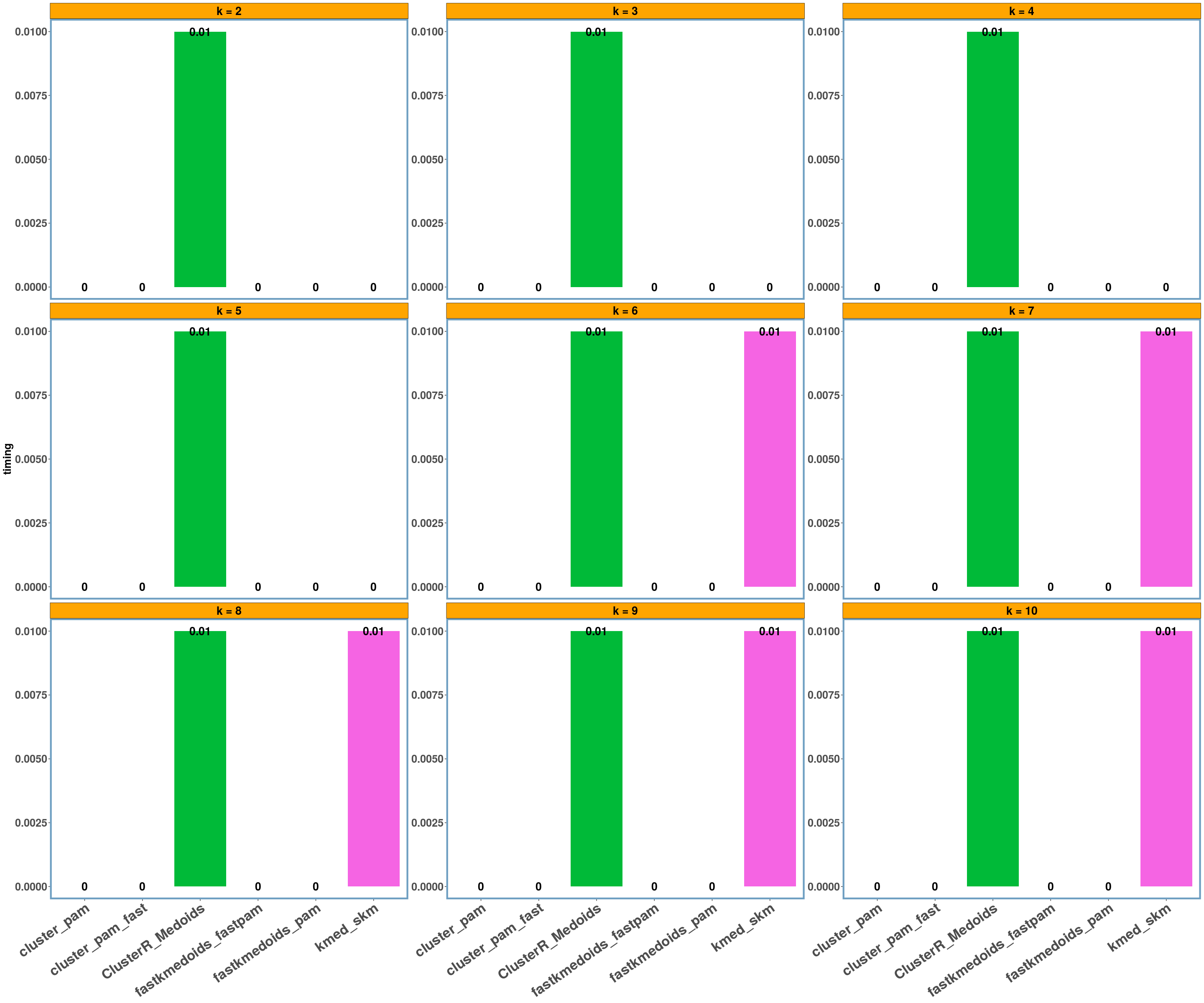
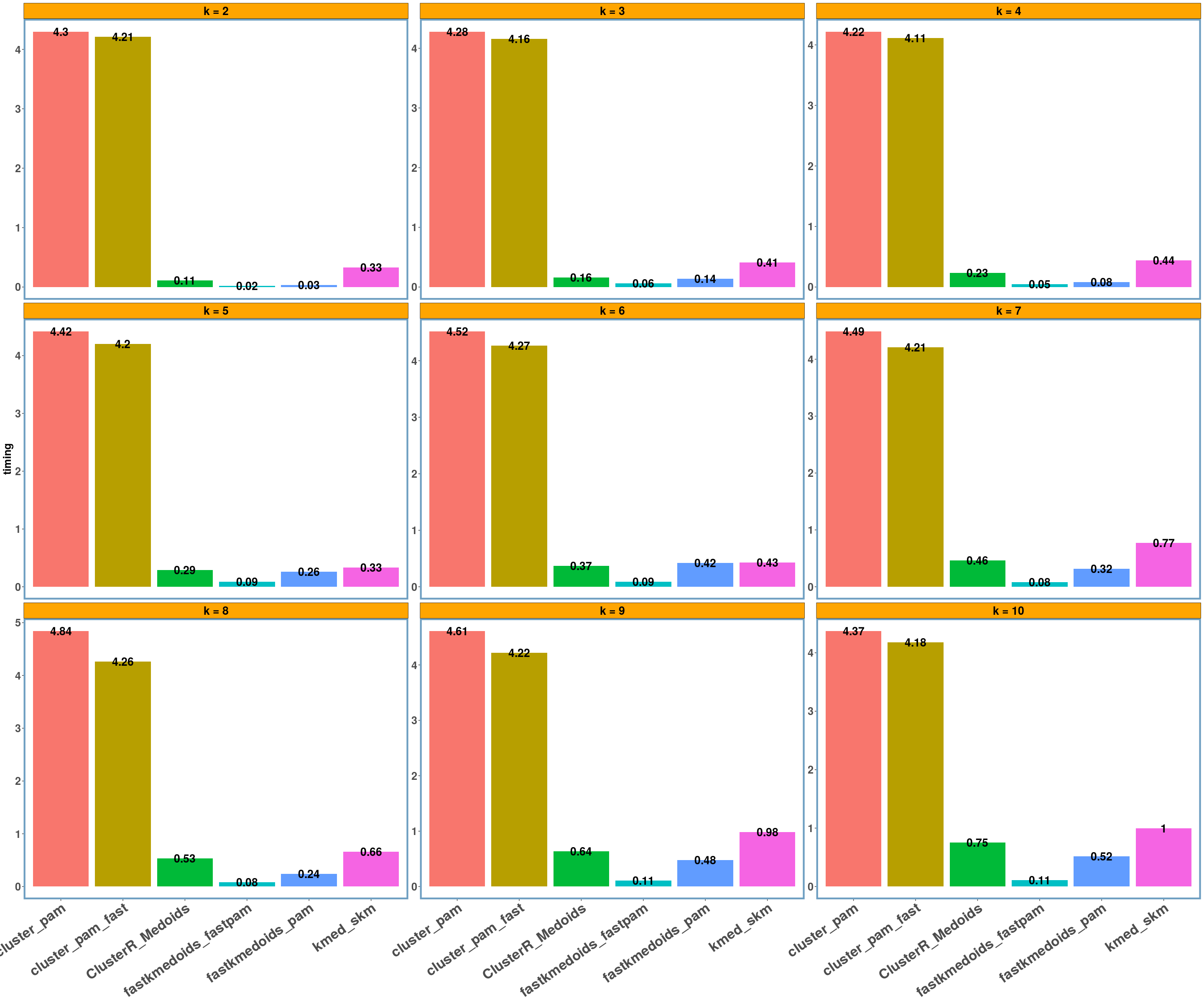
y_axis = 'timing'

data_name = 'rnorm_data'
multi_plot_data(data_index = lst_all[[data_name]], y_column = y_axis)
dietary_survey_IBS dataset
data_name = 'dietary_survey_IBS'
multi_plot_data(data_index = lst_all[[data_name]], y_column = y_axis)
soybean dataset
data_name = 'soybean'
multi_plot_data(data_index = lst_all[[data_name]], y_column = y_axis)
agriculture dataset
data_name = 'agriculture'
multi_plot_data(data_index = lst_all[[data_name]], y_column = y_axis)
geospatial dataset
data_name = 'geospatial'
multi_plot_data(data_index = lst_all[[data_name]]$results, y_column = y_axis)
Conclusions
- Using different datasets and a range of values for k (from 2 to 10) we see that even the exact algorithm does not always give the lowest dissimilarity cost. Moreover, there is a difference in the dissimilarity cost for the different ‘k’ values and the included ‘datasets’ between the various implementations. This probably has to do with the fact that the majority of these implementations are approximate and also differently implemented.
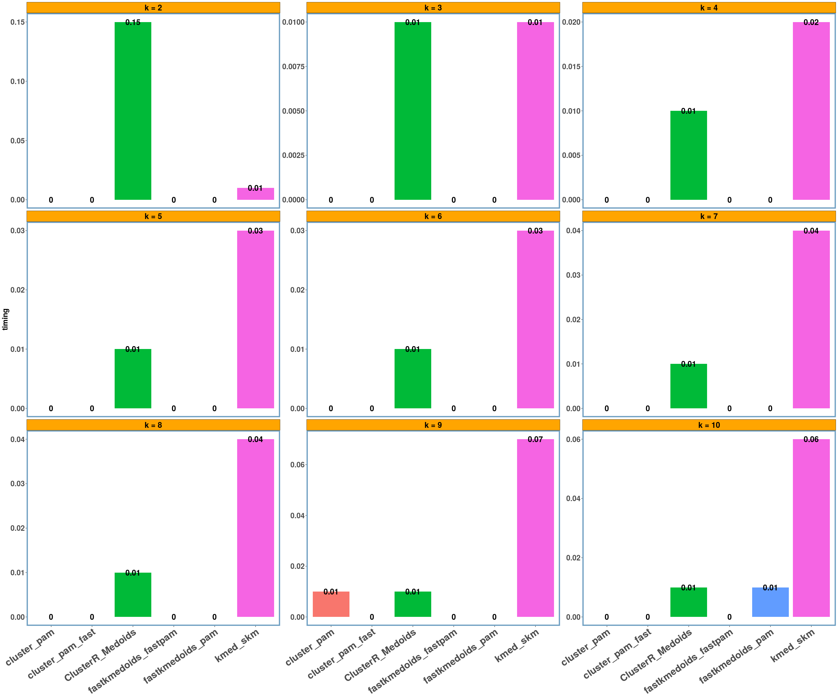
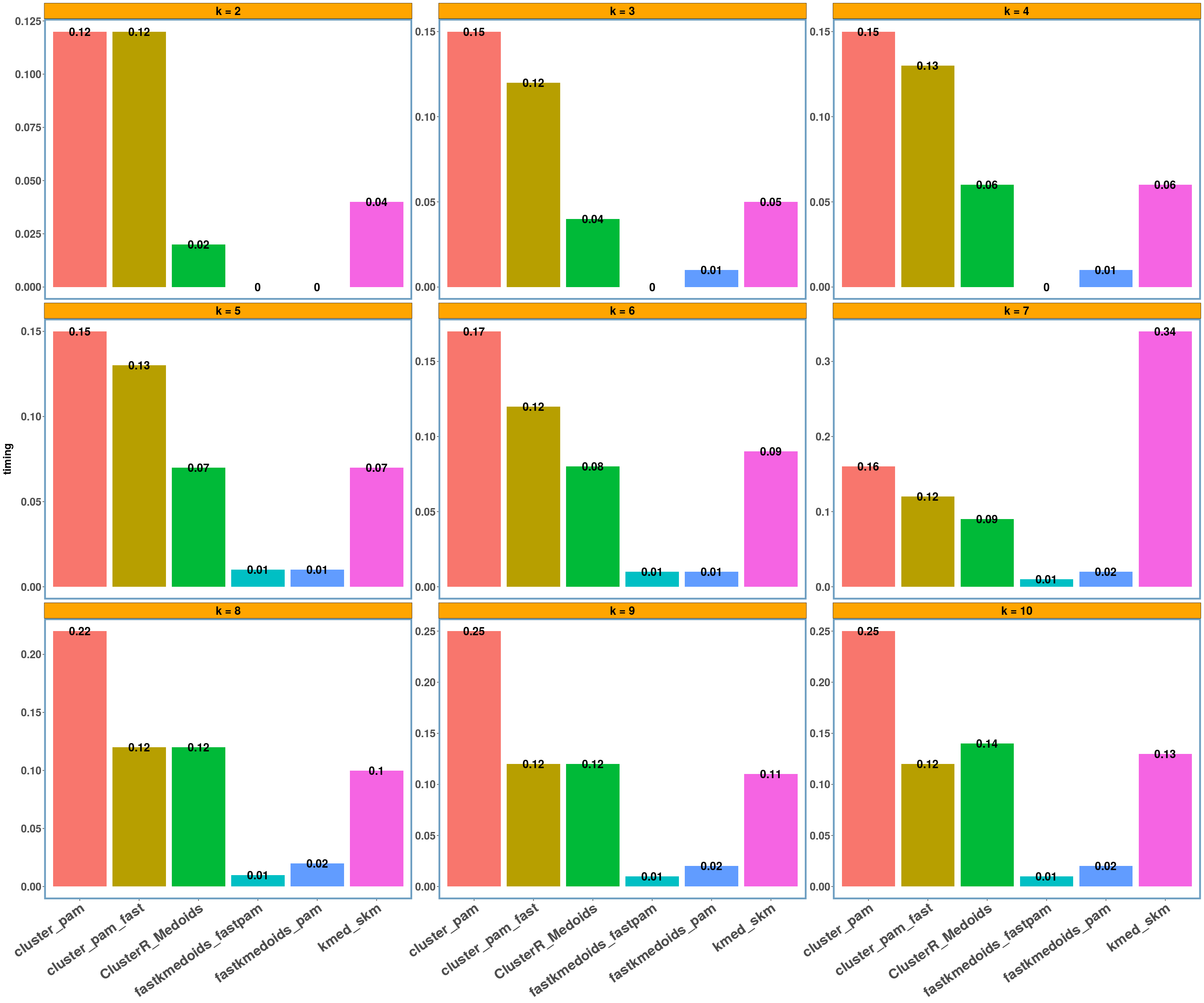
- Regarding the elapsed time the bar-plots show that the fastkmedoids::fastpam() function returns the results faster (compared to the other implementations) in all cases and this is more obvious in the ‘geospatial’ dataset where we have a medium sized dataset consisting of 1000 observations.
Notes
All ‘Partition Around Medoid’ functions take a dissimilarity matrix as input and not the initial input data, therefore the elapsed time does not include the computation of the dissimilarity (or distance) matrix.