
Text Processing using the textTinyR package
05 Jan 2017This blog post is about my recently released package on CRAN, textTinyR. The following notes and examples are based mainly on the package Vignette.
The advantage of the textTinyR package lies in its ability to process big text data files in batches efficiently. For this purpose, it offers functions for splitting, parsing, tokenizing and creating a vocabulary. Moreover, it includes functions for building either a document-term matrix or a term-document matrix and extracting information from those (term-associations, most frequent terms). Lastly, it embodies functions for calculating token statistics (collocations, look-up tables, string dissimilarities) and functions to work with sparse matrices. The source code is based mainly on C++11 and exported in R through the Rcpp, RcppArmadillo and BH packages.
update (04-04-2018): boost-locale is no longer a system requirement for the textTinyR package
The following classes (based on the R6 package) and functions are part of the package:
classes
| big_tokenize_transform | sparse_term_matrix | token_stats |
|---|---|---|
| big_text_splitter() | Term_Matrix() | path_2vector() |
| big_text_parser() | Term_Matrix_Adjust() | freq_distribution() |
| big_text_tokenizer() | term_associations() | print_frequency() |
| vocabulary_accumulator() | most_frequent_terms() | count_character() |
| print_count_character() | ||
| collocation_words() | ||
| print_collocations() | ||
| string_dissimilarity_matrix() | ||
| look_up_table() | ||
| print_words_lookup_tbl() |
functions
| sparse_matrices | tokenization | utilities |
|---|---|---|
| dense_2sparse() | tokenize_transform_text() | bytes_converter() |
| load_sparse_binary() | tokenize_transform_vec_docs() | cosine_distance() |
| matrix_sparsity() | dice_distance() | |
| save_sparse_binary() | levenshtein_distance() | |
| sparse_Means() | read_characters() | |
| sparse_Sums() | read_rows() | |
| text_file_parser() | ||
| utf_locale() | ||
| vocabulary_parser() |
big_tokenize_transform class
The big_tokenize_transform class can be utilized to process big data files and I’ll illustrate this using the english wikipedia pages and articles (to download the data use the following web-address : https://dumps.wikimedia.org/enwiki/latest/enwiki-latest-pages-articles.xml.bz2). The size of the file (after downloading and extracting locally) is aproximalely 59.4 GB and it’s of type .xml (to reproduce the results one needs to have free hard drive space of approx. 200 GB).
Xml files have a tree structure and one should use queries to acquire specific information. First, I’ll observe the structure of the .xml file by using the utility function read_rows(). The read_rows() function takes a file as input and by specifying the rows argument it returns a subset of the file. It doesn’t load the entire file in memory, but it just opens the file and reads the specific number of rows,
library(textTinyR)


PATH = 'enwiki-latest-pages-articles.xml'


subset = read_rows(input_file = PATH, read_delimiter = "\n",

                   rows = 100,

                   write_2file = "/subs_output.txt")
# data subset : subs_output.txt


<mediawiki xmlns="http://www.mediawiki.org/xml/export-0.10/" xmlns:xsi="http://www.w3.org/2001/XMLSchema-instance" xsi:schemaLocation="http://www.mediawiki.org/xml/export-0.10/ http://www.mediawiki.org/xml/export-0.10.xsd" version="0.10" xml:lang="en">
  <siteinfo>
    <sitename>Wikipedia</sitename>
    <dbname>enwiki</dbname>
    <base>https://en.wikipedia.org/wiki/Main_Page</base>
    <generator>MediaWiki 1.28.0-wmf.23</generator>
    <case>first-letter</case>
    <namespaces>
      <namespace key="-2" case="first-letter">Media</namespace>
      <namespace key="-1" case="first-letter">Special</namespace>
      <namespace key="0" case="first-letter" />
      <namespace key="1" case="first-letter">Talk</namespace>
      <namespace key="2" case="first-letter">User</namespace>
      <namespace key="3" case="first-letter">User talk</namespace>
      <namespace key="4" case="first-letter">Wikipedia</namespace>
      <namespace key="5" case="first-letter">Wikipedia talk</namespace>
      <namespace key="6" case="first-letter">File</namespace>
      <namespace key="7" case="first-letter">File talk</namespace>
      <namespace key="8" case="first-letter">MediaWiki</namespace>
.
.
.
    </namespaces>
  </siteinfo>
  <page>
    <title>AccessibleComputing</title>
    <ns>0</ns>
    <id>10</id>
    <redirect title="Computer accessibility" />
    <revision>
      <id>631144794</id>
      <parentid>381202555</parentid>
      <timestamp>2014-10-26T04:50:23Z</timestamp>
      <contributor>
        <username>Paine Ellsworth</username>
        <id>9092818</id>
      </contributor>
      <comment>add [[WP:RCAT|rcat]]s</comment>
      <model>wikitext</model>
      <format>text/x-wiki</format>
      <text xml:space="preserve">#REDIRECT [[Computer accessibility]]

</text>
      <sha1>4ro7vvppa5kmm0o1egfjztzcwd0vabw</sha1>
    </revision>
  </page>
  <page>
    <title>Anarchism</title>
    <ns>0</ns>
    <id>12</id>
    <revision>
      <id>746687538</id>
      <parentid>744318951</parentid>
      <timestamp>2016-10-28T22:43:19Z</timestamp>
      <contributor>
        <username>Eduen</username>
        <id>7527773</id>
      </contributor>
      <minor />
      <comment>/* Free love */</comment>
      <model>wikitext</model>
      <format>text/x-wiki</format>
      <text xml:space="preserve">
In that way one has a picture of the .xml tree structure and can continue by performing queries. The initial data file is too big to fit in the memory of a PC, thus it has to be split in smaller files, pre-processed and then returned as a single file. The main aim of the big_text_splitter() method is to split the data in smaller files of (approx.) equal size by either using the batches parameter or if the file has a structure by adding the end_query parameter too. Here I’ll take advantage of both the batches and the end_query parameters for this task, because I’ll use queries to extract the text tree-elements, so I don’t want that the file is split arbitrarily. Each sub-element in the file begins and ends with the same key-word, i.e. text,
btt = big_tokenize_transform$new(verbose = TRUE)

btt$big_text_splitter(input_path_file = PATH,             # path to the enwiki data file

                  output_path_folder = "/enwiki_spl_data/",  # folder to save the files

                  end_query = '</text>',    # splits the file taking into account the key-word

                  batches = 40,                           # split file in 40 batches (files)

                  trimmed_line = FALSE,                   # the lines will be trimmed

                  verbose = TRUE)
approx. 10 % of data pre-processed
approx. 20 % of data pre-processed
approx. 30 % of data pre-processed
approx. 40 % of data pre-processed
approx. 50 % of data pre-processed
approx. 60 % of data pre-processed
approx. 70 % of data pre-processed
approx. 80 % of data pre-processed
approx. 90 % of data pre-processed
approx. 100 % of data pre-processed

It took 42.7098 minutes to complete the splitting
After the data is split and saved in the output_path_folder (“/ewiki_spl_data/”) the next step is to extract the text tree-elements from the batches by using the big_text_parser() method. The latter takes as arguments the previously created input_path_folder, an output_path_folder to save the resulted text files, a start_query, an end_query, the min_lines (only subsets of text with more than or equal to this minimum will be kept) and the trimmed_line ( specifying if each line is already trimmed both-sides ),
btt$big_text_parser(input_path_folder = "/enwiki_spl_data/", # the previously created folder

                    output_path_folder = "/enwiki_parse/",  # folder to save the parsed files

                    start_query = "<text xml:space=\"preserve\">",  # starts to extract text

                    end_query = "</text>",                        # stop to extract once here

                    min_lines = 1,

                    trimmed_line = TRUE,

                    verbose = TRUE)
====================
batch 1 begins ...
====================

approx. 10 % of data pre-processed
approx. 20 % of data pre-processed
approx. 30 % of data pre-processed
approx. 40 % of data pre-processed
approx. 50 % of data pre-processed
approx. 60 % of data pre-processed
approx. 70 % of data pre-processed
approx. 80 % of data pre-processed
approx. 90 % of data pre-processed
approx. 100 % of data pre-processed

It took 0.296151 minutes to complete the preprocessing

It took 0.0525948 minutes to save the pre-processed data

.
.
.
.

====================
batch 40 begins ...
====================

approx. 10 % of data pre-processed
approx. 20 % of data pre-processed
approx. 30 % of data pre-processed
approx. 40 % of data pre-processed
approx. 50 % of data pre-processed
approx. 60 % of data pre-processed
approx. 70 % of data pre-processed
approx. 80 % of data pre-processed
approx. 90 % of data pre-processed
approx. 100 % of data pre-processed

It took 1.04127 minutes to complete the preprocessing

It took 0.0448579 minutes to save the pre-processed data

It took 40.9034 minutes to complete the parsing
Here, it’s worth mentioning that the big_text_parser is more efficient if it extracts big chunks of text, rather than one-liners. In case of one-line text queries it has to check line by line the whole file, which is inefficient especially for files equal to the enwiki size.
By extracting the text chunks from the data the .xml file size reduces to (approx.) 48.9 GB. One can now continue utilizing the big_text_tokenizer() method in order to tokenize and transform the data. This method takes the following parameters:
batches (each file can be further split in batches during tokenization), to_lower (convert to lower case), to_upper (convert to upper case), utf_locale (change utf locale depending on the language), read_file_delimiter (the delimiter to use for the input data, for instance a tab-delimiter or a new-line delimiter), remove_char (remove specific characters from the text), remove_punctuation_string (remove punctuation before the data is split), remove_punctuation_vector (remove punctuation after the data is split), remove_numbers (remove numbers from the data), trim_token (trim the tokens both-sides), split_string (split the string), split_separator (token split seprator where multiple delimiters can be used), remove_stopwords (remove stopwords using one of the available languages or by providing a user defined vector of words), language (the language of use), min_num_char (the minimum number of characters to keep), max_num_char (the maximum number of characters to keep), stemmer (stemming of the words using either the porter_2steemer or n-gram stemming – those two methods will be explained in the tokenization function), min_n_gram (minimum n-grams), max_n_gram (maximum n-grams), skip_n_gram (skip n-gram), skip_distance (skip distance for n-grams), n_gram_delimiter (n-gram delimiter), concat_delimiter (concatenation of the data in case that one wants to save the file), path_2folder (specified folder to save the data), stemmer_ngram (in case of n-gram stemming the n-grams), stemmer_gamma (in case of n-gram stemming the gamma parameter), stemmer_truncate (in case of n-gram stemming the truncation parameter), stemmer_batches (in case of n-gram stemming the batches parameter ), threads (the number of cores to use in parallel ), save_2single_file (should the output data be saved in a single file), increment_batch_nr (the enumeration of the output files will start from this number), vocabulary_path_file (should a vocabulary be saved in a separate file).
More information about those parameters can be found in the package documentation.
In this blog post I’ll continue using the following transformations:
- conversion to lowercase
- trim each line
- split each line using multiple delimiters
- remove the punctuation ( once splitting is taken place )
- remove the numbers from the tokens
- limit the output words to a specific number of characters
- remove the english stopwords
- and save both the data (to a single file) and the vocabulary files (to a folder).
Each initial file will be split in additional batches to limit the memory usage during the tokenization and transformation phase,
btt$big_text_tokenizer(input_path_folder = "/enwiki_parse/",   # the previously parsed data

                       batches = 4,     # each single file will be split further in 4 batches

                       to_lower = TRUE, trim_token = TRUE,

                       split_string=TRUE, max_num_char = 100,

                       split_separator = " \r\n\t.,;:()?!//",

                       remove_punctuation_vector = TRUE,

                       remove_numbers = TRUE,

                       remove_stopwords = TRUE,

                       threads = 4,

                       save_2single_file = TRUE,      # save to a single file

                       vocabulary_path_folder = "/enwiki_vocab/",  # path to vocabulary folder

                       path_2folder="/enwiki_token/",   # folder to save the transformed data

                       verbose = TRUE)
====================================
transformation of file 1 starts ...
====================================

-------------------
batch 1 begins ...
-------------------

input of the data starts ...
conversion to lower case starts ...
removal of numeric values starts ...
the string-trim starts ...
the split of the character string and simultaneously the removal of the punctuation in the vector starts ...
stop words of the english language will be used
the removal of stop-words starts ...
character strings with more than or equal to 1 and less than 100 characters will be kept ...
the vocabulary counts will be saved in: /enwiki_vocab/batch1.txt
the pre-processed data will be saved in a single file in: /enwiki_token/

-------------------
batch 2 begins ...
-------------------

input of the data starts ...
conversion to lower case starts ...
removal of numeric values starts ...
the string-trim starts ...
the split of the character string and simultaneously the removal of the punctuation in the vector starts ...
stop words of the english language will be used
the removal of stop-words starts ...
character strings with more than or equal to 1 and less than 100 characters will be kept ...
the vocabulary counts will be saved in: /enwiki_vocab/batch1.txt
the pre-processed data will be saved in a single file in: /enwiki_token/

.
.
.
.

====================================
transformation of file 40 starts ...
====================================

-------------------
batch 1 begins ...
-------------------

input of the data starts ...
conversion to lower case starts ...
removal of numeric values starts ...
the string-trim starts ...
the split of the character string and simultaneously the removal of the punctuation in the vector starts ...
stop words of the english language will be used
the removal of stop-words starts ...
character strings with more than or equal to 1 and less than 100 characters will be kept ...
the vocabulary counts will be saved in: /enwiki_vocab/batch40.txt
the pre-processed data will be saved in a single file in: /enwiki_token/

-------------------
batch 2 begins ...
-------------------

input of the data starts ...
conversion to lower case starts ...
removal of numeric values starts ...
the string-trim starts ...
the split of the character string and simultaneously the removal of the punctuation in the vector starts ...
stop words of the english language will be used
the removal of stop-words starts ...
character strings with more than or equal to 1 and less than 100 characters will be kept ...
the vocabulary counts will be saved in: /enwiki_vocab/batch40.txt
the pre-processed data will be saved in a single file in: /enwiki_token/

.
.
.
.

It took 111.689 minutes to complete tokenization
In total, it took approx. 195 minutes (or 3.25 hours) to pre-process (including tokenization, transformation and vocabulary extraction) the 59.4 GB of the enwiki data.
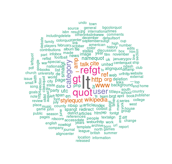
word cloud
Having a clean single text file of all the wikipedia pages and articles one can perform many tasks. For instance, one can build a wordcloud (using the wordcloud package) from the accumulated words (a word of caution : the memory consumption when running the vocabulary_accumulator method for this kind of data size can exceed the 10 GB),
init$vocabulary_accumulator(input_path_folder = "/enwiki_vocab/",

                            vocabulary_path_file = "/VOCAB.txt",

                            max_num_chars = 50)
vocabulary.of.batch 40 will.be.merged ...	minutes.to.merge.sort.batches: 4.57273

	minutes.to.save.data: 0.48584
The following table shows the first rows of the vocabulary counts,
| terms | frequency |
|---|---|
| lt | 111408435L |
| refgt | 49197149L |
| quot | 48688082L |
| gt | 47466149L |
| user | 32042007L |
| category | 30619748L |
| www | 25358252L |
| http | 23008243L |
before plotting the wordcloud, I’ll limit the vocabulary to the first 200 words,
rdr_vocab = textTinyR::read_rows(input_file = "/VOCAB.txt", read_delimiter = "\n",

                                 rows = 200,

                                 write_2file = "/vocab_subset_200terms.txt")

# read the reduced data

vocab_sbs <- readr::read_delim("/vocab_subset_200terms.txt", "\t",

                               escape_double = FALSE, col_names = FALSE,

                               trim_ws = TRUE)

# create the wordcloud

pal2 <- RColorBrewer::brewer.pal(8, "Dark2")

wordcloud::wordcloud(words = vocab_sbs$X1, freq = vocab_sbs$X2,

                     scale = c(4.5, 0.8), random.order = FALSE,

                     rot.per = .15, colors = pal2)
word vectors
UPDATE 11-04-2019: There is an updated version of the fastText R package which includes all the features of the ported fasttext library. Therefore the old fastTextR repository is archived. See also the corresponding blog-post.
I’m currently interested in word vectors and that’s why I also made R-wrappers for the GloVe and the fastText word representation algorithms. The latter two reside in my Github account as separate repositories (GloveR and fastTextR) and can be installed using the install_github function of the devtools package (devtools::install_github(‘mlampros/GloveR’), devtools::install_github(‘mlampros/fastTextR’)).
“A word representation is a mathematical object associated with each word, often a vector. Each dimension’s value corresponds to a feature and might even have a semantic or grammatical interpretation, so we call it a word feature. Conventionally, supervised lexicalized NLP approaches take a word and convert it to a symbolic ID, which is then transformed into a feature vector using a one-hot representation: The feature vector has the same length as the size of the vocabulary, and only one dimension is on.”
Currently, there are many resources on the web on how to use pre-trained word vectors (embeddings) as input to neural networks.
In this blog post I’ll use only the fastTextR word representation algorithm, however detailed documentation and system requirements on how to use either the GloveR or the fastTextR can be found in the corresponding repository. If I would train the whole data file (32.2 GB) using the fastTextR wrapper, it would take (approx.) 15 hours,
library(fastTextR)

skp = skipgram_cbow(input_path = "/output_token_single_file.txt", thread = 4, dim = 50,

                    output_path = "/model", method = "skipgram", verbose = 2)
Read 4018M words
Number of words:  12827221
Number of labels: 0
Progress: 0.2%  words/sec/thread: 89664  lr: 0.099841  loss: 1.055581  eta: 15h32m  14m
thus, just for illustration purposes I’ll limit the train data to approx. 1 GB of the output file,
reduced_data = read_characters(input_file = "/output_token_single_file.txt",

                               characters = 1000000000,        # approx. 1 GB of the data

                               write_2file = "/reduced_single_file.txt")


skp = skipgram_cbow(input_path = "/reduced_single_file.txt",  # reduced data set

                    output_path = "/model",                # saves model and word vectors

                    dim = 50,                              # 50-dimensional word vectors

                    method = "skipgram",                   # method = 'skipgram'

                    thread = 4, verbose = 2)
Read 124M words
Number of words:  5029370
Number of labels: 0
Progress: 100.0%  words/sec/thread: 94027  lr: 0.000000  loss: 0.186674  eta: 0h0m

time to complete : 33.53577 mins
the following vector-subset is the example output of the “model.vec” file, which includes the 50-dimensional word vectors,
lt 0.12207 0.16117 0.4641 0.73876 0.43968 0.63911 -0.53747 0.1398 .....
refgt -0.0038898 -0.13976 0.26077 0.7775 0.2228 0.28169 -0.48306 .....
quot 0.7295 -0.12472 0.32131 0.46965 0.45363 0.85022 -0.051471 .....
gt 0.41287 0.26584 0.6612 0.78185 0.46692 0.74092 -0.23816 .....
cite 0.037943 0.095684 0.62832 0.93794 0.19776 0.44592 -0.21641 .....
www -0.31855 0.42268 0.3875 1.5457 -0.23804 0.34022 -0.051849 .....
ref 0.45236 -0.21766 0.6341 0.76392 0.53734 0.66976 -0.23162 .....
http -0.42692 0.48637 0.28622 1.7019 -0.25739 0.25948 -0.026582 .....
namequot 0.56828 -0.30782 0.45707 0.78346 0.53727 0.62445 .....
– -0.010281 0.25528 0.04708 0.49679 0.043934 0.33733 -0.42706 .....
amp 0.06308 0.11968 0.11885 0.67699 -0.11448 0.25183 -0.48789 .....
category -1.5705 -0.40638 0.61064 2.5691 -0.52987 0.68096 .....
county -0.85743 0.071625 -0.43393 0.17157 -0.32874 1.771 .....
org -0.26974 0.76983 0.57599 1.5939 -0.1706 0.21937 -0.44645 .....
states -0.40973 -0.48528 0.092905 0.011603 -0.035727 0.52807 .....
united -0.25079 -0.49813 0.070942 0.16762 0.069961 0.56868 .....
web -0.066578 0.14837 0.23088 1.2919 -0.252 0.31441 -0.3799 .....
census -0.29033 -0.73695 0.35474 -0.5237 -0.15206 1.7089 .....
.
.
.
sparse_term_matrix class
The sparse_term_matrix class includes methods for building a document-term or a term-document matrix and extracting information from those matrices (it relies on RcppArmadillo and can handle large sparse matrices too). I’ll explain all the different methods using a toy text file downloaded from wikipedia,
The term planet is ancient, with ties to history, astrology, science, mythology, and religion. Several planets in the Solar System can be seen with the naked eye. These were regarded by many early cultures as divine, or as emissaries of deities. As scientific knowledge advanced, human perception of the planets changed, incorporating a number of disparate objects. In 2006, the International Astronomical Union (IAU) officially adopted a resolution defining planets within the Solar System. This definition is controversial because it excludes many objects of planetary mass based on where or what they orbit.
Although eight of the planetary bodies discovered before 1950 remain planets under the modern definition, some celestial bodies, such as Ceres, Pallas, Juno and Vesta (each an object in the solar asteroid belt), and Pluto (the first trans-Neptunian object discovered), that were once considered planets by the scientific community, are no longer viewed as such.
The planets were thought by Ptolemy to orbit Earth in deferent and epicycle motions. Although the idea that the planets orbited the Sun had been suggested many times, it was not until the 17th century that this view was supported by evidence from the first telescopic astronomical observations, performed by Galileo Galilei.
At about the same time, by careful analysis of pre-telescopic observation data collected by Tycho Brahe, Johannes Kepler found the planets orbits were not circular but elliptical. As observational tools improved, astronomers saw that, like Earth, the planets rotated around tilted axes, and some shared such features as ice caps and seasons. Since the dawn of the Space Age, close observation by space probes has found that Earth and the other planets share characteristics such as volcanism, hurricanes, tectonics, and even hydrology.
Planets are generally divided into two main types: large low-density giant planets, and smaller rocky terrestrials. Under IAU definitions, there are eight planets in the Solar System. In order of increasing distance from the Sun, they are the four terrestrials, Mercury, Venus, Earth, and Mars, then the four giant planets, Jupiter, Saturn, Uranus, and Neptune. Six of the planets are orbited by one or more natural satellites.
The sparse_term_matrix class can be initialized using either a vector of documents or a text file. Assuming the downloaded file is saved as “planets.txt”, then a document-term-matrix can be created in the following way,
init = sparse_term_matrix$new(vector_data = NULL,          # in case of vector of documents

                              file_data = "/planets.txt",     # input the .txt data

                              document_term_matrix = TRUE)   # document term matrix as output


tm = init$Term_Matrix(sort_terms = TRUE,      # initial terms are sorted

                      to_lower = TRUE,          # convert to lower case

                      trim_token = TRUE,        # trim token

                      split_string = TRUE,      # split string

                      tf_idf = TRUE,            # tf-idf will be returned

                      verbose = TRUE)
minutes.to.tokenize.transform.data: 0.00001	total.time: 0.00001

Warning message:
empty character strings present in the column names they will be replaced with proper characters
tm


5 x 212 sparse Matrix of class "dgCMatrix"
   [[ suppressing 91 column names ‘X’, ‘X17th’, ‘X1950’ ... ]]

[1,] -0.001939591 .         .          0.009747774 0.01949555   ......
[2,] -0.003255742 .         0.01636233 .           .            ......
[3,] -0.003440029 0.0172885 .          .           .            ......
[4,] -0.002196645 .         .          .           .            ......
[5,] -0.002681199 .         .          .           .          . ......

[1,] 0.007121603 .          0.009747774 .          0.005434315 . ......
[2,] 0.007969413 0.01636233 .           .          .           . ......
[3,] .           .          .           .          0.009638219 . ......
[4,] 0.008065430 .          .           0.01103965 .             ......
[5,] .           .          .           .          .             ......

[1,] -0.001939591 0.009747774 .          .          .           ......
[2,] -0.003255742 .           .          .          0.01636233  ......
[3,] -0.010320088 .           .          .          .           ......
[4,] -0.006589936 .           0.01103965 0.01103965 .           ......
[5,] -0.002681199 .           .          .          .           ......
.
.
.
The Term_Matrix method takes almost the same parameters as the ( already explained ) big_text_tokenizer() method. The only differences are:
- sort_terms ( should the output terms - rows or columns depending on the document_term_matrix parameter - be sorted in alphabetical order )
- print_every_rows ( verbose output intervalls )
- normalize ( applies l1 or l2 normalization )
- tf_idf ( the term-frequency-inverse-document-frequency will be returned )
Details about the parameters of the Term_Matrix method can be found in the package documentation.
To adjust the sparsity of the output matrix one can take advantage of the Term_Matrix_Adjust method, (by adjusting the sparsity_thresh parameter towards 0.0 a proportion of the sparse terms will be removed)
res_adj = init$Term_Matrix_Adjust(sparsity_thresh = 0.6) # terms (here columns) which sum to zero will be removed
res_adj


5 x 9 sparse Matrix of class "dgCMatrix"
          planets           by            X       solar          and          as  ......
[1,] -0.005818773 -0.001939591 -0.001939591 0.004747735 -0.001939591 0.007121603  ......
[2,] -0.006511484 -0.003255742 -0.003255742 0.003984706 -0.006511484 0.007969413  ......
[3,] -0.006880059 -0.010320088 -0.003440029 .           -0.003440029 .            ......
[4,] -0.006589936 -0.006589936 -0.002196645 .           -0.008786581 0.008065430  ......
[5,] -0.013405997 -0.002681199 -0.002681199 0.003281523 -0.008043598 .            ......
The term_associations method returns the correlation of specific terms (Terms) with all the other terms in the output matrix. The dimensions of the output matrix can vary depending on which one of the Term_Matrix, Term_Matrix_Adjust is run previously. In the previous step I adjusted the initial sparse matrix using a sparsity_thresh of 0.6, thus the new dimensions will be,
dim(res_adj)

[1] 5 9
and the resulted terms,
init$term_associations(Terms = c('planets', 'by', 'INVALID'), keep_terms = NULL, verbose = TRUE)
the ' INVALID ' term does not exist in the terms vector

total.number.variables.processed:   2	minutes.to.complete: 0.00000

$planets
     term correlation
 1:    as  0.65943196
 2:   and  0.48252671
 3:     X  0.07521813
 4:    by -0.26301349
 5:    of         NaN
 6: solar -0.11887462
 7:  were         NaN
 8:   the -0.15500900
 9:   in.         NaN
10:  that  0.44307617
11: earth -0.24226093

$by
       term correlation
 1:   solar   0.9092777
 2:       X   0.5010034
 3: planets  -0.2630135
 4:      of         NaN
 5:    were         NaN
 6:     the   0.7838436
 7:      as   0.3698239
 8:     and  -0.0594149
 9:     in.         NaN
10:   earth  -0.6952757
11:    that  -0.9338884
Lastly, the most_frequent_terms method gives the frequency of the terms in the corpus. However, the function returns only if the normalize parameter is NULL and the tf_idf parameter is FALSE ( those two parameters belong to the init$Term_Matrix() method ),
init = sparse_term_matrix$new(file_data = "/planets.txt", document_term_matrix = TRUE)

tm = init$Term_Matrix(sort_terms = TRUE,

                      to_lower = TRUE,

                      trim_token = TRUE,

                      split_string = TRUE,

                      tf_idf = FALSE,            # disable tf-idf

                      verbose = TRUE)


init$most_frequent_terms(keep_terms = 10, threads = 1, verbose = TRUE)
minutes.to.complete: 0.00000


        term frequency
 1:     the        28
 2: planets        15
 3:     and        11
 4:      of         9
 5:      by         9
 6:      as         8
 7:     in.         6
 8:       X         5
 9:     are         5
10:    that         5
More information about the sparse_term_matrix class can be found in the package documentation.
token_stats class
The token_stats class can be utilized to output corpus statistics. Each of the following methods can take either a vector of terms, a text file or a folder of files as input:
- path_2vector : is a helper method which takes a path to a file or folder of files and returns the content in form of a vector,
init = token_stats$new(path_2file = "/planets.txt")    # input the 'planets.txt' file

vec = init$path_2vector()
[1] "The term planet is ancient, with ties to history, astrology, science, mythology, and religion. Several planets in the Solar System can be seen with the naked eye. These were regarded by many early cultures as divine, or as emissaries of deities. As scientific knowledge advanced, human perception of the planets changed, incorporating a number of disparate objects" ....

[2] "Although eight of the planetary bodies discovered before 1950 remain" ....
.
.
- freq_distribution : it returns a named-unsorted vector frequency distribution for a vocabulary file
# assuming the following 'freq_vocab.txt'

the
term
planet
is
ancient
with
ties
to
history
astrology
science
mythology
and
religion
several
planets
in
the
solar
system
can
be
seen
with
the
naked
eye
these
were
this method would return,
init = token_stats$new(path_2file = 'freq_vocab.txt')

init$freq_distribution()

init$print_frequency(subset = NULL)
        words freq
 1:       the    3
 2:      with    2
 3:   ancient    1
 4:       and    1
 5: astrology    1
 6:        be    1
 7:       can    1
 8:       eye    1
 9:   history    1
10:        in    1
11:        is    1
12: mythology    1
13:     naked    1
14:    planet    1
15:   planets    1
16:  religion    1
17:   science    1
18:      seen    1
19:   several    1
20:     solar    1
21:    system    1
22:      term    1
23:     these    1
24:      ties    1
25:        to    1
26:      were    1
        words freq
- count_character : it returns the number of characters for each word of the corpus.
for the previously mentioned ‘freq_vocab.txt’ it would output,
  init = token_stats$new(path_2file = 'freq_vocab.txt')

  vec_tmp = init$count_character()

  init$print_count_character(number = 3)
# words with number of characters equal to 3

[1] "the" "and" "the" "can" "the" "eye"
- collocation_words : it returns a co-occurence frequency table for n-grams. “A collocation is defined as a sequence of two or more consecutive words, that has characteristics of a syntactic and semantic unit, and whose exact and unambiguous meaning or connotation cannot be derived directly from the meaning or connotation of its components”. The input to the function should be text n-grams separated by a delimiter ( for instance the tokenize_transform_text() function in the next code chunk will build n_grams of length 3 ),
# the data needs to be n-grams thus first tokenize and build the n-grams using
# the 'tokenize_transform_text' function ( the "planets.txt" file as input )

tok = tokenize_transform_text("planets.txt",

                              to_lower = T,

                              split_string = T,

                              min_n_gram = 3,

                              max_n_gram = 3,

                              n_gram_delimiter = "_")

init = token_stats$new(x_vec = tok$token)      # vector data as input

vec_tmp = init$collocation_words()
the example output of the vec_tmp vector is,
[1] ""       "17th"       "1950"    "2006"    "a"     "about"   "adopted"   "advanced"
[9] "age"    "although" ....
.
.
.
and the print_collocations method returns the coolocations for the example word ancient,
res = init$print_collocations(word = "ancient")
    is   with   ties planet
 0.333  0.333  0.167  0.167
- string_dissimilarity_matrix : it returns a string-dissimilarity-matrix using either the dice, levenshtein or cosine distance. The input can be a character string vector only. In case that the method is dice then the dice-coefficient (similarity) is calculated between two strings for a specific number of character n-grams ( dice_n_gram ). The dice and levenshtein methods are applied to words, whereas the cosine distance to word-sentences.
For illustration purposes I’ll use the previously mentioned ‘freq_vocab.txt’ file, but first I have to convert the text file to a character vector,
# first initialization of token_stats

init = token_stats$new(path_2file = 'freq_vocab.txt')

tmp_vec = init$path_2vector()      # convert to vector


# second initialization to compute the dissimilarity matrix

init_tok = token_stats$new(x_vec = tmp_vec)

res = init_tok$string_dissimilarity_matrix(dice_n_gram = 2, method = "dice",

                                          split_separator = " ", dice_thresh = 1.0,

                                          upper = TRUE, diagonal = TRUE, threads = 1)
                the      term    planet is   ancient      with      ties to   history ....
the       0.0000000 0.7777778 1.0000000  1 1.0000000 0.7777778 0.7777778  1 1.0000000 ....
term      0.7777778 0.0000000 1.0000000  1 1.0000000 1.0000000 0.8000000  1 1.0000000 ....
planet    1.0000000 1.0000000 0.0000000  1 0.7333333 1.0000000 1.0000000  1 1.0000000 ....
is        1.0000000 1.0000000 1.0000000  0 1.0000000 1.0000000 1.0000000  0 1.0000000 ....
ancient   1.0000000 1.0000000 0.7333333  1 0.0000000 1.0000000 0.8461538  1 1.0000000 ....
with      0.7777778 1.0000000 1.0000000  1 1.0000000 0.0000000 1.0000000  1 1.0000000 ....
ties      0.7777778 0.8000000 1.0000000  1 0.8461538 1.0000000 0.0000000  1 1.0000000 ....
to        1.0000000 1.0000000 1.0000000  0 1.0000000 1.0000000 1.0000000  0 1.0000000 ....
history   1.0000000 1.0000000 1.0000000  1 1.0000000 1.0000000 1.0000000  1 0.0000000 ....
astrology 1.0000000 1.0000000 1.0000000  1 0.8888889 1.0000000 1.0000000  1 0.7777778 ....
science   0.8333333 1.0000000 1.0000000  1 0.5000000 1.0000000 0.8461538  1 1.0000000 ....
.
.
.
here by adjusting (reducing ) the dice_thresh parameter we can force values close to 1.0 to become 1.0,
init_tok = token_stats$new(x_vec = tmp_vec)

res = init_tok$string_dissimilarity_matrix(dice_n_gram = 2, method = "dice",

                                           split_separator = " ", dice_thresh = 0.6,

                                           upper = TRUE, diagonal = TRUE, threads = 1)
          the term planet is ancient with ties to history astrology science ....
the       0.0    1    1.0  1     1.0    1    1  1       1       1.0     1.0 ....
term      1.0    0    1.0  1     1.0    1    1  1       1       1.0     1.0 ....
planet    1.0    1    0.0  1     1.0    1    1  1       1       1.0     1.0 ....
is        1.0    1    1.0  0     1.0    1    1  0       1       1.0     1.0 ....
ancient   1.0    1    1.0  1     0.0    1    1  1       1       1.0     0.5 ....
with      1.0    1    1.0  1     1.0    0    1  1       1       1.0     1.0 ....
ties      1.0    1    1.0  1     1.0    1    0  1       1       1.0     1.0 ....
to        1.0    1    1.0  0     1.0    1    1  0       1       1.0     1.0 ....
history   1.0    1    1.0  1     1.0    1    1  1       0       1.0     1.0 ....
astrology 1.0    1    1.0  1     1.0    1    1  1       1       0.0     1.0 ....
science   1.0    1    1.0  1     0.5    1    1  1       1       1.0     0.0 ....
.
.
.
- look_up_table : The idea here is to split the input words to n-grams using a numeric value and then retrieve the words which have a similar character n-gram.
It returns a look-up-list where the list-names are the n-grams and the list-vectors are the words associated with those n-grams. The words for each n-gram can be retrieved using the print_words_lookup_tbl method. The input can be a character string vector only.
# first initialization of token_stats

init = token_stats$new(path_2file = 'freq_vocab.txt')

tmp_vec = init$path_2vector()    # convert to vector


# second initialization to compute the look-up-table

init_lk = token_stats$new(x_vec = tmp_vec)

is_vec = init_lk$look_up_table(n_grams = 3)
# example output for the 'is_vec' vector

[1] ""    "ake" "_an" "anc" "ane" "_as" "ast" "cie" "eli" "enc" "era" "eve" .....
[29] "net" "ola" "olo" "_pl" "pla" "_re" "rel" "rol" "_sc" "sci" "_se" "see" .....
[57] "tro" "ver" "_we" "wer" "_wi" "wit" "yst" "yth"
then retrieve words with same n-grams,
init_lk$print_words_lookup_tbl(n_gram = "log")
"_astrology_" "_mythology_"
the underscores are necessary to distinguish the begin and end of each word when computing the n-grams.
More information about the token_stats class can be found in the package documentation.
helper functions for sparse_matrices
The purpose of creating those functions is because I observed that they return faster in comparison to other R packages. The following code chunks explain each one of the functions,
#---------------------------------
# conversion from dense to sparse
#---------------------------------

library(textTinyR)

set.seed(1)
dsm = matrix(sample(0:1, 100, replace = T), 10, 10)

res_sp = dense_2sparse(dsm)

res_sp
## 10 x 10 sparse Matrix of class "dgCMatrix"
##
##  [1,] . . 1 . 1 . 1 . . .
##  [2,] . . . 1 1 1 . 1 1 .
##  [3,] 1 1 1 . 1 . . . . 1
##  [4,] 1 . . . 1 . . . . 1
##  [5,] . 1 . 1 1 . 1 . 1 1
##  [6,] 1 . . 1 1 . . 1 . 1
##  [7,] 1 1 . 1 . . . 1 1 .
##  [8,] 1 1 . . . 1 1 . . .
##  [9,] 1 . 1 1 1 1 . 1 . 1
## [10,] . 1 . . 1 . 1 1 . 1
#-------------
# column- sums
#-------------

sm_cols = sparse_Sums(res_sp, rowSums = FALSE)

sm_cols
## [1] 6 5 3 5 8 3 4 5 3 6
#----------
# row-sums
#----------

sm_rows = sparse_Sums(res_sp, rowSums = TRUE)

sm_rows
## [1] 3 5 5 3 6 5 5 4 7 5
#---------------
# column- means
#---------------

mn_cols = sparse_Means(res_sp, rowMeans = FALSE)

mn_cols
## [1] 0.6 0.5 0.3 0.5 0.8 0.3 0.4 0.5 0.3 0.6
#-----------
# row-means
#-----------

mn_rows = sparse_Means(res_sp, rowMeans = TRUE)

mn_rows
## [1] 0.3 0.5 0.5 0.3 0.6 0.5 0.5 0.4 0.7 0.5
#-------------------------------------
# sparsity of a matrix (as percentage)
#-------------------------------------

matrix_sparsity(res_sp)
## 51.9999 %
#------------------------------------------------------
# saving and loading sparse matrices (in binary format)
#------------------------------------------------------

save_sp = save_sparse_binary(res_sp, file_name = "save_sparse.mat")

load_sp = load_sparse_binary(file_name = "save_sparse.mat")
More information about the helper functions for sparse matrices can be found in the package documentation.
tokenization
The tokenize_transform_text() function applies tokenization and transformation in a similar way to the big_text_tokenizer() method, however for small to medium data sets. The input can be either a character string (text data) or a path to a file. This method takes as input a single character string (character-string == of length one). The parameters for the tokenize_transform_text() function are the same to the (already explained) big_text_tokenizer() method with the only exception being the input data type.
The tokenize_transform_vec_docs() function works in the same way to the Term_Matrix() method and it targets small to medium data sets. It takes as input a vector of documents and retains their order after tokenization and transformation has taken place. Both the tokenize_transform_text() and tokenize_transform_vec_docs() share the same parameters, with the following two exceptions,
- the object is a character vector
- the as_token parameter : if TRUE then the output of the function is a list of (split) token. Otherwise it’s a vector of character strings (sentences)
The following code chunks give an overview of the mentioned functions,
#------------------------
# tokenize_transform_text
#------------------------


# example input : "planets.txt"


res_txt = tokenize_transform_text(object = "/planets.txt",

                                  to_lower = TRUE,

                                  utf_locale = "",

                                  trim_token = TRUE,

                                  split_string = TRUE,

                                  remove_stopwords = TRUE,

                                  language = "english",

                                  stemmer = "ngram_sequential",

                                  stemmer_ngram = 3,

                                  threads = 1)
the output is a vector of tokens after the english stopwords were removed and the terms were stemmed (ngram_sequential of length 3),
# example output :

$token
  [1] "ter"          "planet"        "anci"         "ties"         "hist"  ...

  [16] "early"        "cultu"        "divi"         "emissar"      "deit" ....

  [31] "object"       "2006"         "internatio"   "astro"        "union" ...

  [46] "exclu"        "object"       "planet"        "mass"         "based"" ....
.
.
.

attr(,"class")
[1] "tokenization and transformation"
#----------------------------
# tokenize_transform_vec_docs
#----------------------------


# the input should be a vector of documents

init = token_stats$new(path_2file = "/planets.txt")

inp = init$path_2vector()   # convert text file to character vector


# run the function using the input-vector

res_dct = tokenize_transform_vec_docs(object = inp,

                                      as_token = FALSE,  # return character vector of documents

                                      to_lower = TRUE,

                                      utf_locale = "",

                                      trim_token = TRUE,

                                      split_string = TRUE,

                                      remove_stopwords = TRUE,

                                      language = "english",

                                      stemmer = "porter2_stemmer",

                                      threads = 1)
the output is a vector of transformed documents after the english stopwords were removed and the terms were stemmed (porter2-stemming),
$token
[1] "term planet ancient tie histori astrolog scienc mytholog religion planet solar ....."

[2] "planetari bodi discov 1950 remain planet modern definit celesti bodi cere palla ....."

[3] "planet thought ptolemi orbit earth defer epicycl motion idea planet orbit sun ....."

[4] "time care analysi pre-telescop observ data collect tycho brahe johann kepler  ....."

[5] "planet general divid main type larg lowdens giant planet smaller rocki terrestri ....."


attr(,"class")
[1] "tokenization and transformation"
The documents can be returned as a list of character vectors by specifying, as_token = TRUE,
# run the function using the input-vector

res_dct_tok = tokenize_transform_vec_docs(object = inp,

                                          as_token = TRUE,

                                          to_lower = TRUE,

                                          utf_locale = "",

                                          trim_token = TRUE,

                                          split_string = TRUE,

                                          remove_stopwords = TRUE,

                                          language = "english",

                                          stemmer = "porter2_stemmer",

                                          threads = 1)
$token
$token[[1]]
 [1] "term"        "planet"    "ancient"  "tie"   "histori"   .....

$token[[2]]
 [1] "planetari"    "bodi"     "discov"   "1950"   "remain"   .....

$token[[3]]
 [1] "planet"       "thought"  "ptolemi"  "orbit"   "earth"   .....


attr(,"class")
[1] "tokenization and transformation"
A few words about the utf_locale, remove_stopwords and stemmer parameters.
- The utf_locale can take as input either an empty string (“”) or a character string (for instance “el_GR.UTF-8”). It should be a non-empty string if the text input is other than english. However, currently for the windows OS only english character strings or files can be input and pre-processed.
- The remove_stopwords parameter can be either a boolean (TRUE, FALSE) or a character vector of user defined stop-words. The available languages are specified by the parameter language. Currently, there is no support for chinese, japanese, korean, thai or languages with ambiguous word boundaries.
- The stemmer parameter can take as input one of the porter2_stemmer, ngram_sequential or ngram_overlap.
- The porter2_stemmer is a C++ implementation of the snowball-porter2 stemming algorithm. The porter2_stemmer applies to all functions of the textTinyR package.
- On the other hand, n-gram stemming is “language independent” and supported by the ngram_sequential and ngram_overlap functions. The n-gram stemming applies to all functions except for the sparse_term_matrix and tokenize_transform_vec_docs functions of the textTinyR package.
- ngram_overlap : The ngram_overlap stemming method is based on N-Gram Morphemes for Retrieval, Paul McNamee and James Mayfield
- ngram_sequential : The ngram_sequential stemming method is a modified version based on Generation, Implementation and Appraisal of an N-gram based Stemming Algorithm, B. P. Pande, Pawan Tamta, H. S. Dhami.
utility functions
The following code chunks illustrate the utility functions of the package (besides the read_characters() and read_rows() which used in the previous code chunks),
#---------------------------------------
# cosine distance between word sentences
#---------------------------------------

s1 = 'sentence with two words'

s2 = 'sentence with three words'

sep = " "

cosine_distance(s1, s2, split_separator = sep)
## [1] 0.75
#------------------------------------------------------------------------
# dice distance between two words (using n-grams -- the lower the better)
#------------------------------------------------------------------------

w1 = 'word_one'

w2 = 'word_two'

n = 2

dice_distance(w1, w2, n_grams = n)
## [1] 0.2857143
#---------------------------------------
# levenshtein distance between two words
#---------------------------------------

w1 = 'word_two'

w2 = 'word_one'

levenshtein_distance(w1, w2)
## [1] 3
#---------------------------------------------
# bytes converter (returns the size of a file)
#---------------------------------------------

PATH = "/planets.txt"

bytes_converter(input_path_file = PATH, unit = "KB" )
## [1] 2.213867
#---------------------------------------------------
# returns the utf-locale for the available languages
#---------------------------------------------------


utf_locale(language = "english")
## [1] "en.UTF-8"
#-----------------
# text file parser
#-----------------

# The text file should have a structure (such as an xml-structure), so that
# subsets can be extracted using the "start_query" and "end_query" parameters.
# (it works similarly to the big_text_parser() method, however for small to medium sized files)

# example input "example_file.xml" file :

<?xml version="1.0"?>
<sked>
  <version>2</version>
  <flight>
    <carrier>BA</carrier>
    <number>4001</number>
    <date>2011-07-21</date>
  </flight>
  <flight cancelled="true">
    <carrier>BA</carrier>
    <number>4002</number>
    <date>2011-07-21</date>
  </flight>
</sked>
fp = text_file_parser(input_path_file = "example_file.xml",

                      output_path_file = "/output_folder/example_output_file.txt",

                      start_query = '<number>', end_query = '</number>',

                      min_lines = 1, trimmed_line = FALSE)
"example_output_file.txt" :

4001
4002
#------------------
# vocabulary parser
#------------------

# the 'vocabulary_parser' function extracts a vocabulary from a structured text (such as
# an .xml file) and works in the exact same way as the 'big_tokenize_transform' class,
# however for small to medium sized data files


pars_dat = vocabulary_parser(input_path_file = '/folder/input_data.txt',

                             start_query = 'start_word', end_query = 'end_word',

                             vocabulary_path_file = '/folder/vocab.txt',

                             to_lower = TRUE, split_string = TRUE,

                             remove_stopwords = TRUE)
An updated version of the textTinyR package can be found in my Github repository and to report bugs/issues please use the following link, https://github.com/mlampros/textTinyR/issues.